In this project, we are going to delve into the fundamental operating principles of diffusion models, and understand how does image generation with diffusion models work under the hood. To start off with, we are going to start with the DeepFloyd IF diffusion model. You can find more information about the model here.

To start off, let's see what the DeepFloyd IF model can generate with the precomputed text embeddings - which are numerical representations of text that capture the meaning and context of words. These embeddings allow the model to understand the relationship between text and images by converting words into a format that the model can process mathematically. For this process, we have used the seed:

As you can see, for each prompt, we have created different versions with varying number of inference steps. Inference steps in diffusion models control how gradually the model transforms random noise into a coherent image. With fewer steps (like 9), the process is faster but may produce less refined results. Using more steps (like 50) allows for a more detailed and precise generation process, though it takes longer to compute.

Here are some results generated by the DeepFloyd IF model with the seed=31693169.

prompt: an oil painting of a snowy mountain village

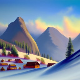
num inference steps: 9

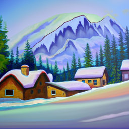
num inference steps: 20

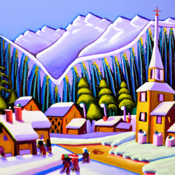
num inference steps: 50

prompt: a man wearing a hat

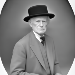
num inference steps: 9

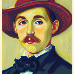
num inference steps: 20

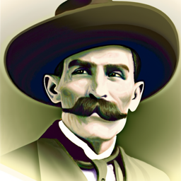
num inference steps: 50

prompt: a rocketship

num inference steps: 9

num inference steps: 20

num inference steps: 50

Sampling Loops

Forward Process

Before we get going with the implementation of the sampling loops, let's understand how the image generation pipeline works under the hood. In order to train our models, we first start off with clean images and then iteratively generate noisy versions of these images until we reach pure noise. Then, a diffusion model's goal is to learn how to reverse this process to generate clean images from pure noise. The diffusion model does so by learning the amount of noise that's added to it's input image through training. Then, during inference, we start off with a random noise pattern and iteratively predict the noise to denoise the initial image, to a point where we refined it to match the input prompt.

As you learned from the above paragh, a key part of the pipeline is to be able to iteratively add noise to the initial clean image. This is achieved through the sampling loop, which we are going to implement from scratch.

In this formula, given the clean image x₀, we get the noised version for timestep t by sampling from a Gaussian distribution with mean \(\sqrt{\bar{\alpha}_t}x_0\) and variance \(1 - \bar{\alpha}_t\).

Now, let's observe some results from our implementation of the sampling loop.

clean image

noised image at timestep 250

noised image at timestep 500

noised image at timestep 750

Classical Denoising

Now that we are able to noise our images, let's work on denoising them. To start off with, let's try the classical denoising approach - gaussian blur.

Gaussian blur is a fundamental image processing technique that smooths out an image by averaging each pixel with its neighboring pixels. The averaging is done using a Gaussian distribution - meaning pixels closer to the center have more influence than those further away. This process effectively reduces noise and detail in the image, as sharp transitions between pixels are softened. Think of it like looking at an image through frosted glass - the details become less distinct and blend together smoothly.

hover over the images to see the noised version

denoised image at timestep 250

denoised image at timestep 500

denoised image at timestep 750

One-step Denoising

Now, instead of gaussian blur we are going to use a pretrained diffusion model to denoise our images.The Unet we are going to use has been trained on a dataset for predicting the amount of noise added to the input image. Therefore, we are going to use it to predict the noise in our noised images. Then, subtract the predicted noise from the noised image to get the denoised image, or as close as we can get to the original clean image.

This model has been trained to predict the noise at a given timestep, therefore, we are going to provide the noised image at time=t and subtract the predicted noise from it to get the denoised image, x_0.

Hover over the images to see the denoised version

denoised image at timestep 250

denoised image at timestep 500

denoised image at timestep 750

In addition to the improved results from gaussian denoising, one interesting artifact is the "change" in imagery for timestep=750. This causes from the fact that we are trying to estimate the clean image from such a noisy image that the model can't get the exact details right, but instead, gets a close approximation from the natural image manifold.

Iterative Denoising

Although the one-step denoising approach has improved the results, it is still not perfect because it's not how diffusion models are designed to work. Diffusion models are designed to iteratively denoise the image. However, the longer the iteration process, the more costly it gets. However, we can speed this by skipping steps.

In that case, for every step, the following is the iterative denoising formula:

$$x_{t'} = \frac{\sqrt{\bar{\alpha}_{t'}\beta_t}}{1 - \bar{\alpha}_t} x_0 + \frac{\sqrt{\alpha_t(1 - \bar{\alpha}_{t'})}}{1 - \bar{\alpha}_t} x_t + v_\sigma$$

where:

• \(x_t\) is image at timestep \(t\)
• \(x_{t'}\) is your noisy at timestep \(t'\) where \(t' < t\) (less noisy)
• \(\bar{\alpha}_{t'}\) is defined by alphas_cumprod, which is the cumulative product of noise scaling factors at each timestep.
• \(\alpha_t = \frac{\bar{\alpha}_t}{\bar{\alpha}_{t'}}\)
• \(\beta_t = 1 - \alpha_t\)
• \(x_0\) estimate of the clean image

In order to generate the below results, we noise the input image up to a certain timestep, not to pure noise. Then, denoise iteratively until we reach timestep=0.

Here are every fifth step of the iterative denoising:

timestep 690

timestep 540

timestep 390

timestep 240

timestep 90

Hover over to compare the denoising results:

Iterative denoising clean estimate

One step denoising clean estimate

Gaussian blur denoising clean estimate

Diffusion Model Sampling

In comparison to the above section, in this section, we are going to see what we can achieve if we start off with pure noise instead partially noised input image. If we start with pure noise, we can sample images according to our conditioning prompt, more on that later in the project. For now, our conditioning signal (prompt) will be a high quality photo.

Here are the results:

Classifier Free Guidance (CFG)

The results above are not great, indeed, some of them doesn't convey any meaning. A method that we can employ to improve our results in a technique called Classifier Free Guidance (CFG).

In the previous section, we based our optimization only on the conditioned noise prediction ε_c. With CFG, we introduce a parameter ε_u, that is the unconditioned noise estimate. We then combine the two with the following formula,

$$ \epsilon = \epsilon_c + \gamma(\epsilon_c - \epsilon_u) $$

As you see, $$\gamma = 0$$ gives us the conditioned noise signal like the above section, $$\gamma = 1$$ gives us the unconditioned noise signal. However, when $$\gamma > 1$$ we then witness the improvements in our results.

Here are couple examples

Image To Image Translation

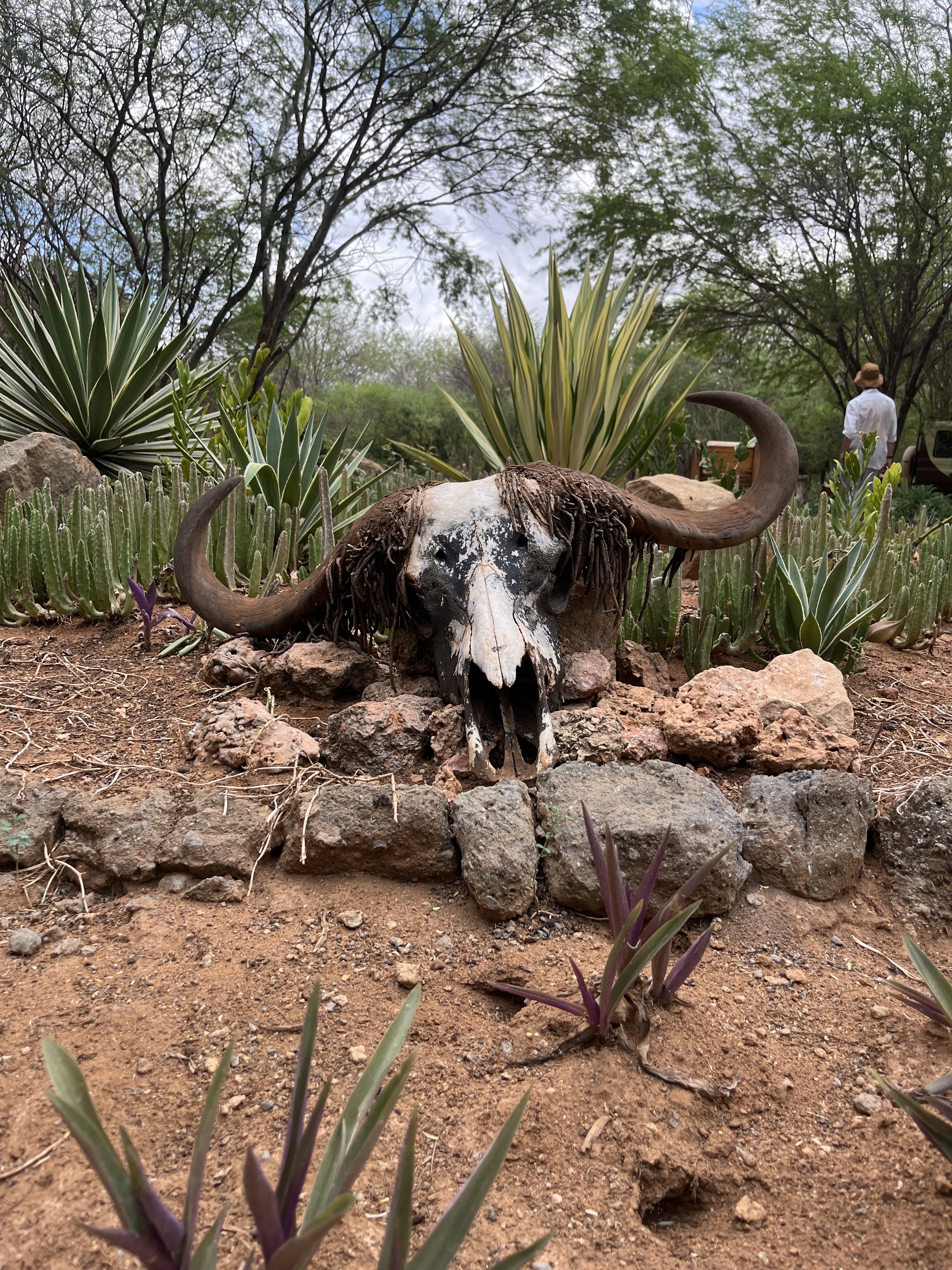
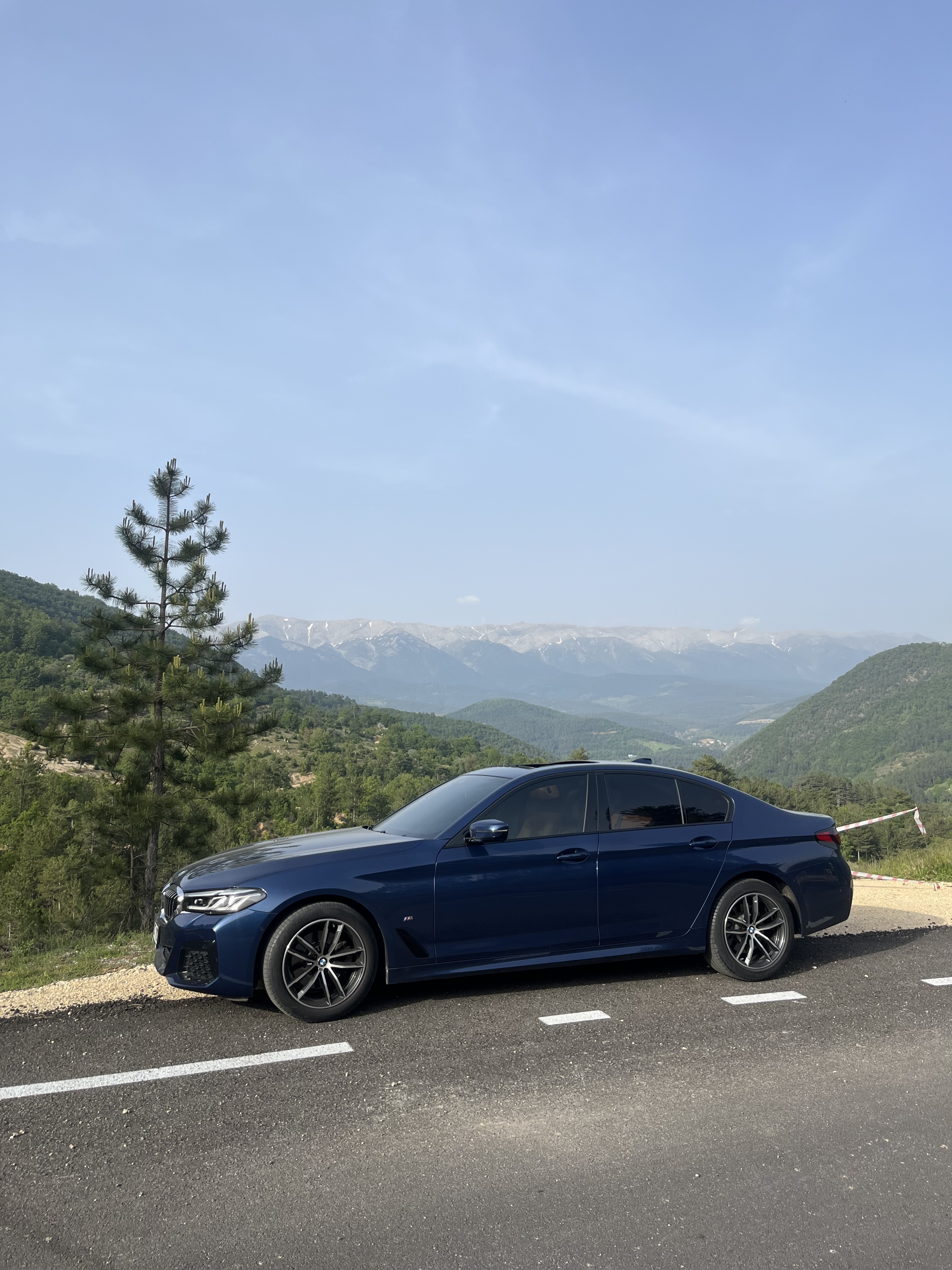
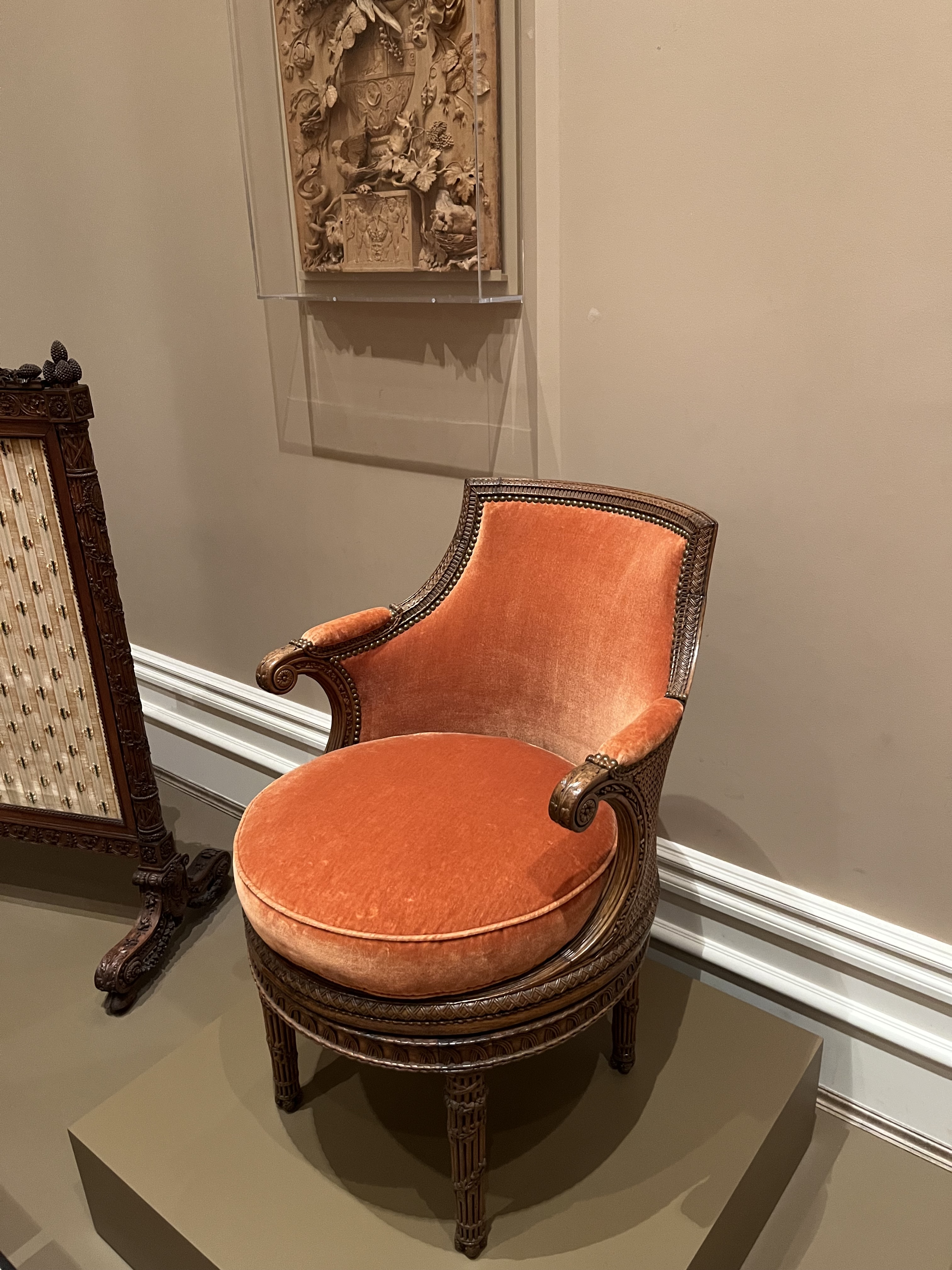
In previous sections, we have noised then denoised the input campanile image, which ended up giving us outputs, in which edits were made on the input image. The reason for that is, from the amount of noise we added to the image, the model is able to only recover a certain amount of details. For the portions that it can't recover, it "hallucinates" the details, in an appropriate manner to force the image to be back on the natural image manifold.

In this section, we are going to observe the results of this "hallucination" process by noising our input image to different amounts and observing the results of the respective denoising processes. Remember, the more noise we add, the more the model hallucinates. The earlier the step is, the more noise we have added.

Input Image

Step 1

Step 3

Step 5

Step 7

Step 10

Step 20

Input Image

Step 1

Step 3

Step 5

Step 7

Step 10

Step 20

Input Image

Step 1

Step 3

Step 5

Step 7

Step 10

Step 20

Input Image

Step 1

Step 3

Step 5

Step 7

Step 10

Step 20

Step 25

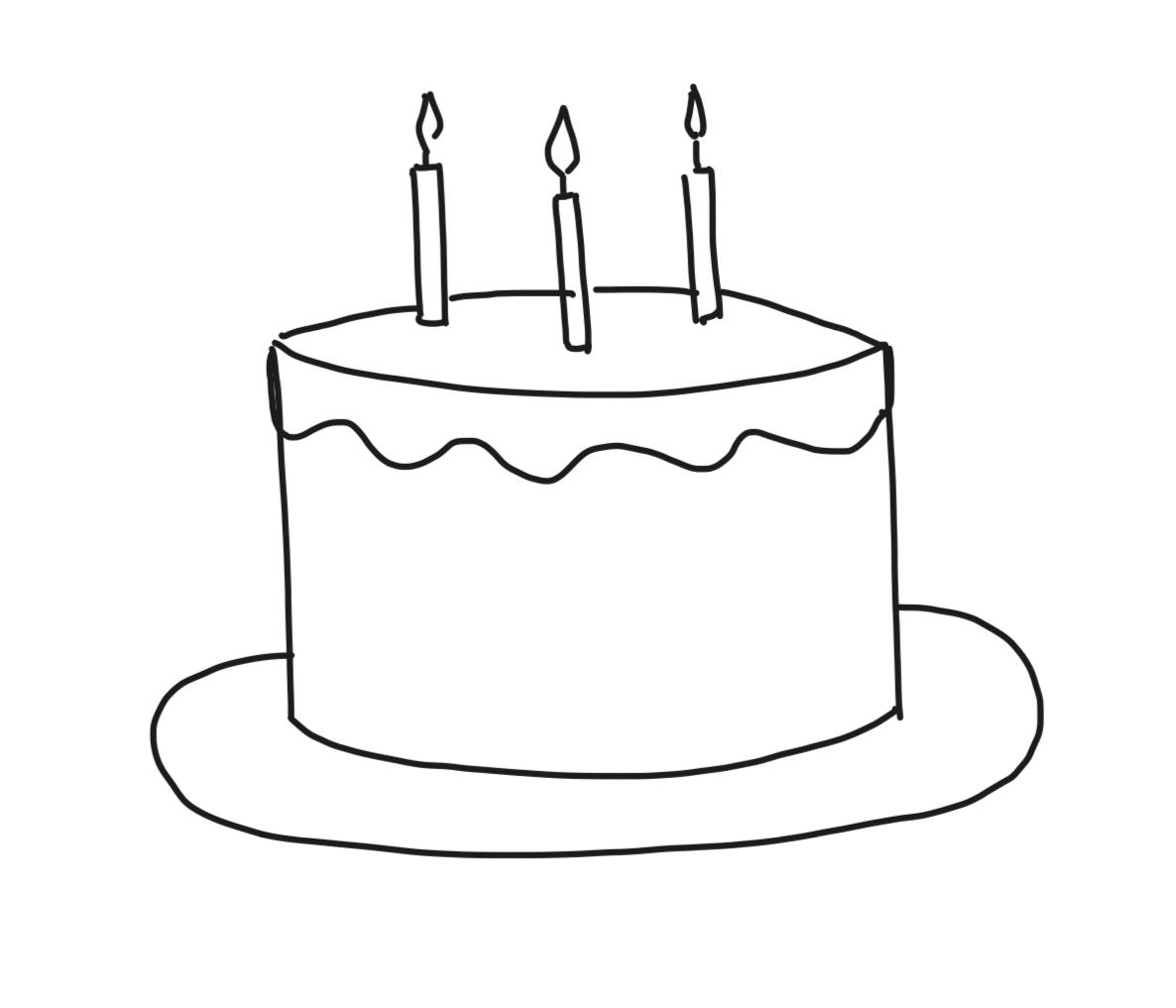
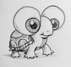
Hand-Drawn Image Translation

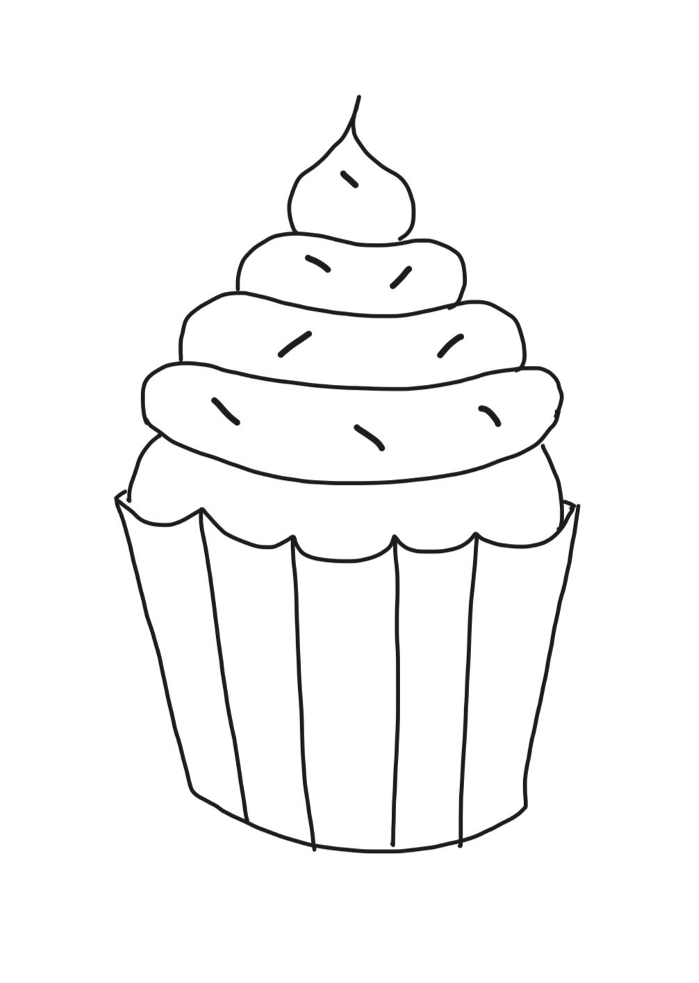
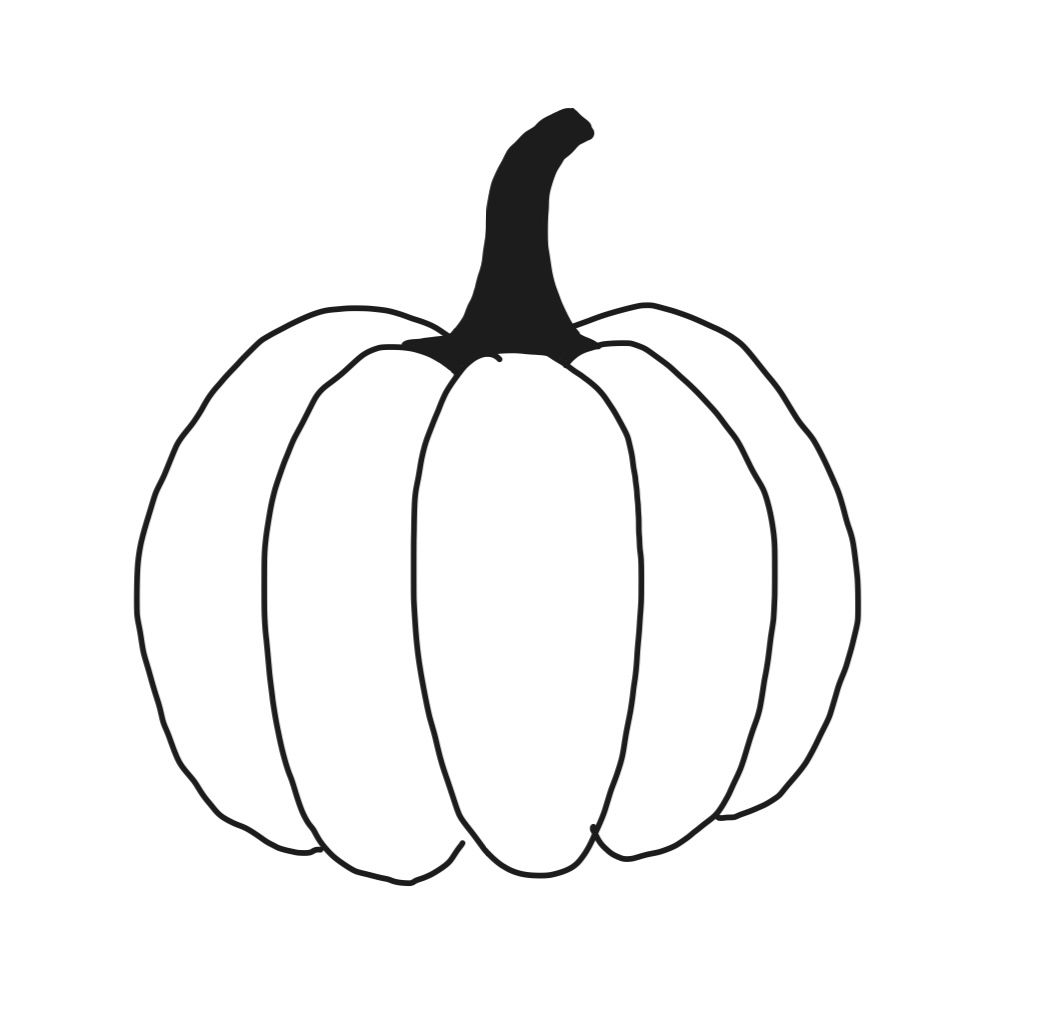
Now we are going to run the same pipeline on non-realistic images instead of realistic inputs to see how the model behaves.

Here are the results:

Input Image

Step 1

Step 3

Step 5

Step 7

Step 10

Step 20

Step 25

Input Image

Step 1

Step 3

Step 5

Step 7

Step 10

Step 20

Step 25

Input Image

Step 1

Step 3

Step 5

Step 7

Step 10

Step 20

Step 25

Step 30

Input Image

Step 1

Step 3

Step 5

Step 7

Step 10

Step 20

Step 25

Inpainting

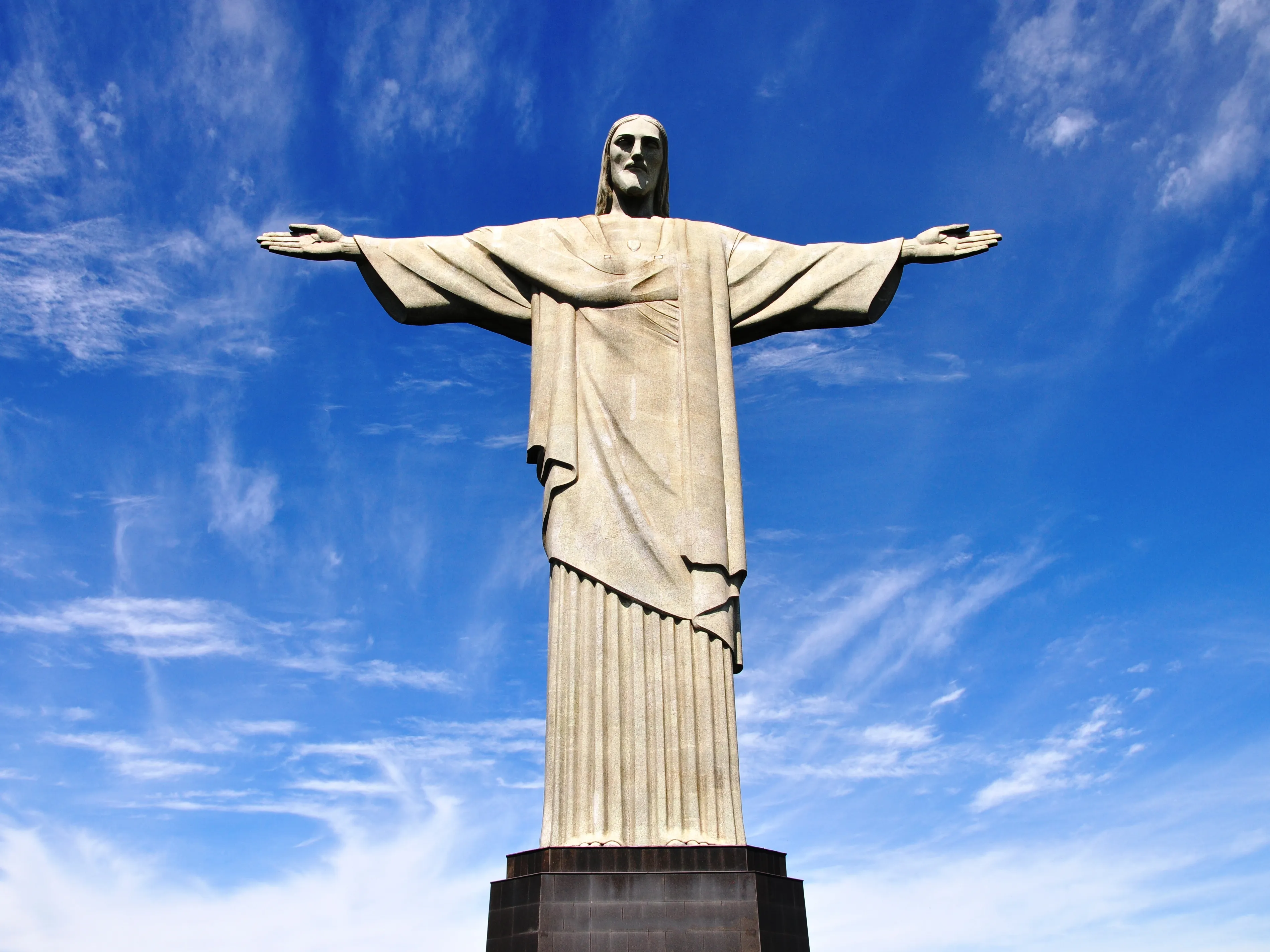
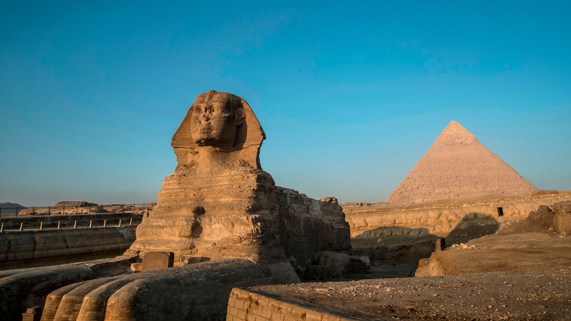
Now, we can use the same pipeline with modifications (to follow the RePaint paper) to implement inpaintings.

That is, given a starting image and a binary mask, we can create new content for the parts of the mask where it's 1, and paste the existing content to the masked out portions. For this, we can use the same pipeline and generate x_t, then, only retreieve the masked out portions. For the rest of the image, we generate the noisy image at the timestep that we are at, and force them on to the current image at t.

Here are the results:

Input Image

Step 10

Step 11

Step 13

Step 15

Step 17

Step 20

Input Image

Step 2

Step 3

Step 5

Step 7

Step 17

Input Image

Step 2

Step 5

Step 7

Step 17

Step 20

Step 23

Text Conditional Image to Image Translation

Now, we will repeat the task in the above Image to Image Translation section. However, this time we won't operate on the unconditioned noise signal, but instead, condition on a text prompt. That's why now we aren't purely projecting on to the natural image manifold, but instead, we are projecting on to a more complex space which is conditioned on the text prompt.

Here are the results:

Prompt: An oil painting of an old man

Input Image

Step 1

Step 3

Step 5

Step 7

Step 10

Step 20

Prompt: A pencil

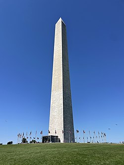
Input Image

Step 1

Step 3

Step 5

Step 7

Step 10

Step 20

Prompt: A rocketship

Input Image

Step 1

Step 3

Step 5

Step 7

Step 10

Step 20

Visual Anagrams

Now, in this part, we are going to creatae optical illusions with diffusion models. Our first illusion will be visual anagrams. That is, images that have two different content encoded when observed from different orientations. For this section, we are going to encode two different images in the two vertical directions. That is, the content observed will be different when the image is flipped vertically.

In order to achieve this, we are going to predict two different noise estimates for the normal and flipped versions of the image respectively. Then, we are going to average them out and then use the averaged error in our optimization.

Here is the formula for the noise prediction:

\[\epsilon_1 = \text{UNet}(x_t, t, p_1)\]

\[\epsilon_2 = \text{flip}(\text{UNet}(\text{flip}(x_t), t, p_2))\]

\[\epsilon = \frac{(\epsilon_1 + \epsilon_2)}{2}\]

Hover over the images to see the flipped version:

an oil painting of people around a campfire

photo of a green flourishing tree

photo of a burning tree

Hybrid Images

Another optical illusion we can create is hybrid images. That is, images were two different content are encoded and interpreted when observed from different distances. This is possible because the different content encoding lies in the lower and higher frequencies of the image respectively. In order to achieve this, we have followed and implemented the Factorized Diffusion paper.

Similar to the above section, we are generating two different error esimations for our two different prompts. Then, we are creating our final error estimation by adding the lower frequencies of one error estimation to the higher frequencies of the other error estimation, and optimizing for the result. We used a gaussian filter as our low pass filter.

Here are the results:

Waterfall from up close, skull from a distance

Bouquet of flowers from up close, a tiger's face from a distance

A cabin in the woods from up close, photo of a man wearing a hat from a distance

Training a Single-Step Denoising UNet

In the previous sections, we have built our pipelines over the abstraction that we had a pre-trained UNet denoiser. Now, we are going to get our hands dirty and train our denoiser. The following is the architecture of the UNet we are going to implement and train.

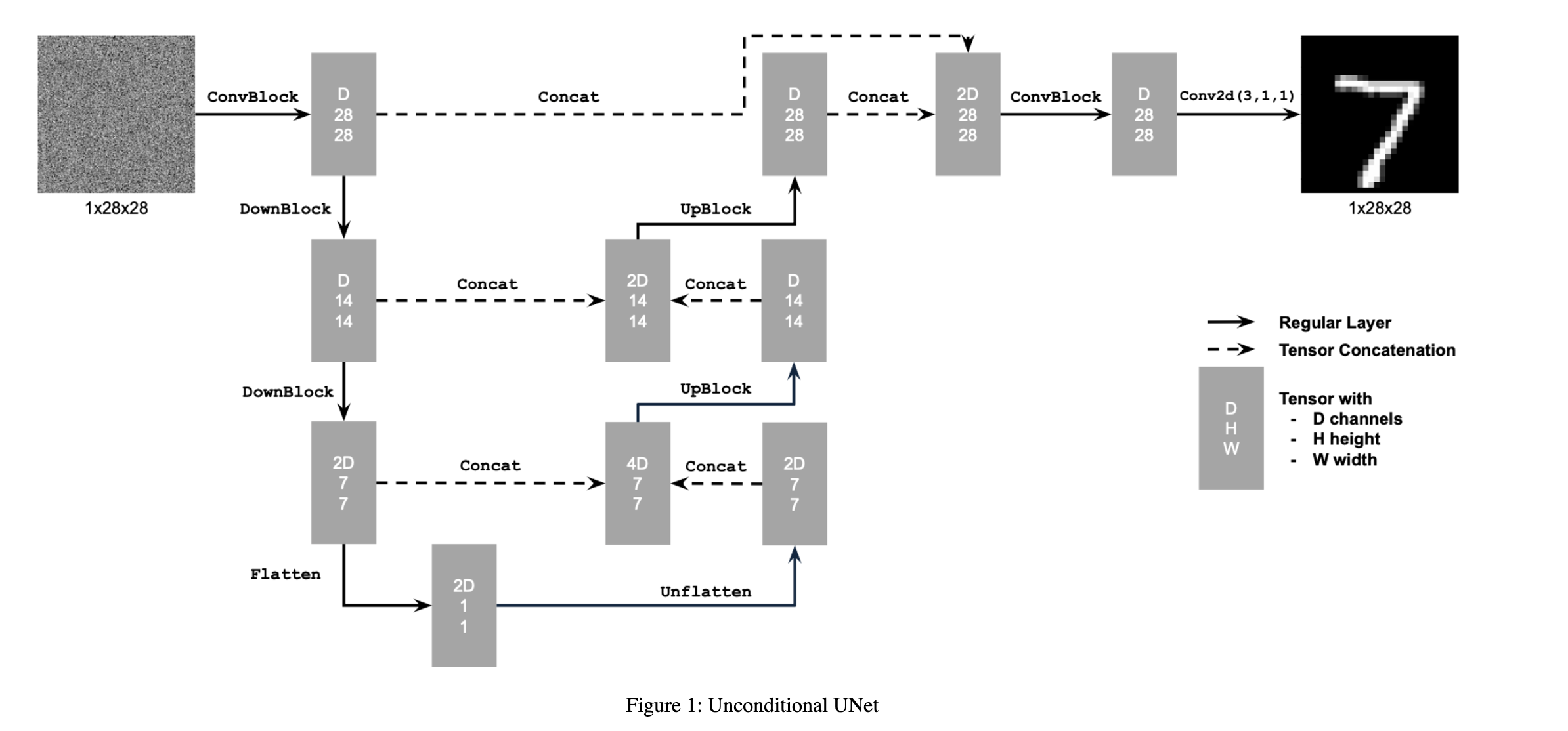
For our training, we are going to optimize over an L2 loss in which we try to minize the distance between the predicted clean image versus the ground truth clean image. We are going to create the noisy images to predict from via adding gaussian noise to clear images from the dataset.

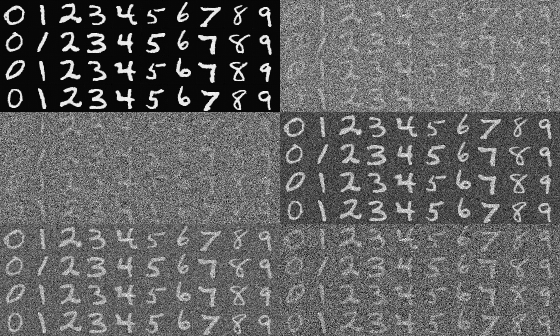
Here are some example images of how the noisy images we generate for training look like:

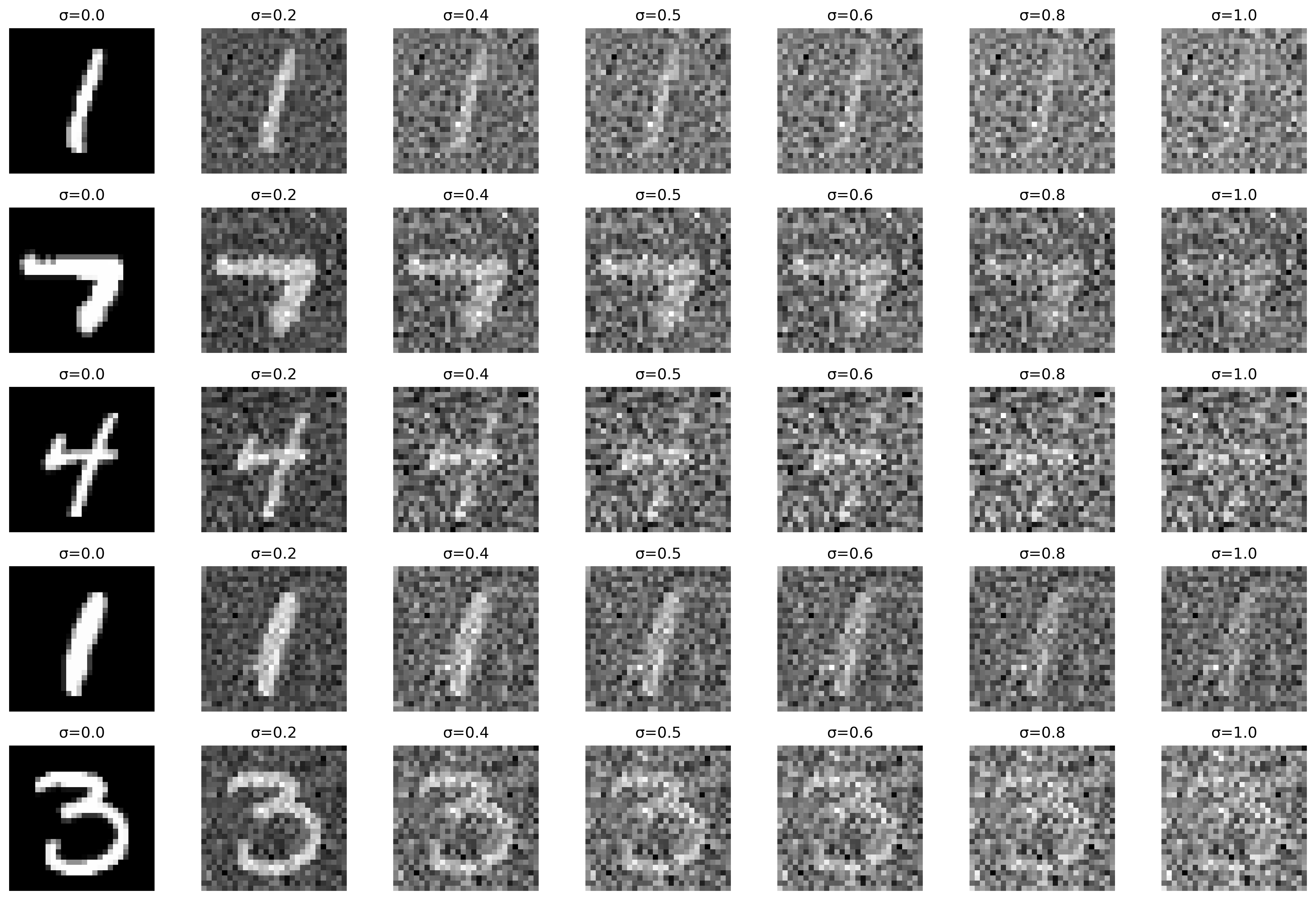
Now, we going to train the UNet for $$\sigma = 0.5$$ with batch size 256, learning rate 1e-4 with the adam optimizer, and with 128 hidden dimensions for 5 epochs.

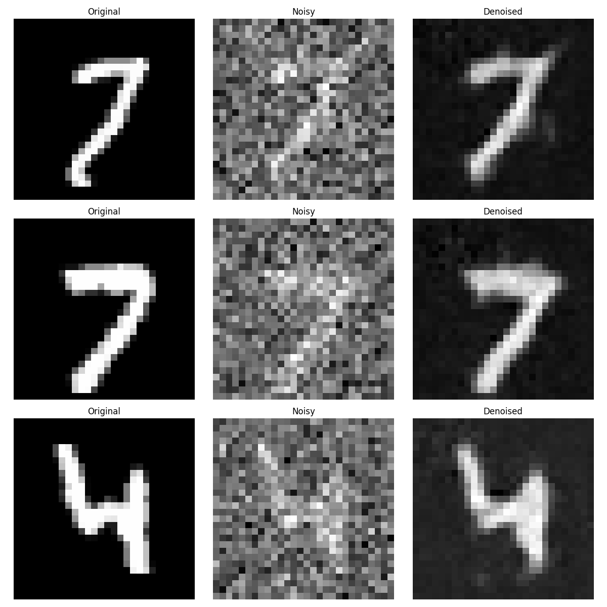
Epoch 1

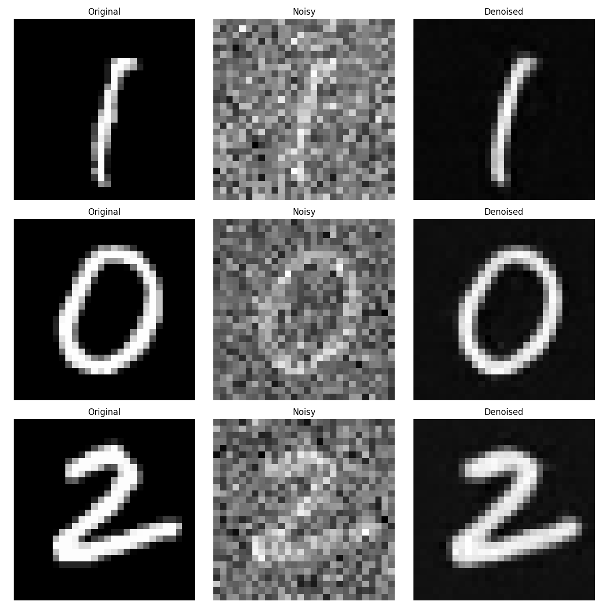
Epoch 5

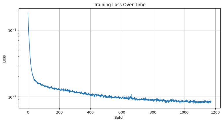
Training Loss Curve

Out Of Distribution Testing

The denoiser we trained in the previous step has been trained for images noised with \(\sigma = 0.5\). Let's see how it performs on images noised with different sigmas.

Training a Diffusion Model

Now that we have our denoiser working, we are ready to implement the diffusion model, following the DDPM paper.

One difference from previous steps is that, now, instead of predicting the clean image with our denoiser, we are going to optimize it over L2 loss again but this time predict the noise added at the given timestep. Then, "subtract" the noise from the image at the timestep to iteratively denoise our image.

The derivation of the image x_t at timestep t is given by:

\[x_t = \sqrt{\bar{\alpha}_t} x_0 + \sqrt{1 - \bar{\alpha}_t} \epsilon\]

where \(\epsilon\) is N(0, 1).

However, our previouly trained UNet was trained for a set noise variance. However, in reality, the noise variance varies with the input t. Therefore, we need to build the notion of time into our model. For that we are going to add time conditioning to our model.

Time Conditioned UNet

Following the course staff suggestion, I have decided to add time conditoning to my existing implementation by adding two fully connected layers that takes the scalar time value and transforms it into a higher-dimensional representation that can be effectively combined with the image features throughout the network. This transformation helps the model understand how much noise to remove at each timestep as model now has a conception of time during training.

The Fully Connected layers inject the conditoning signal into the following part of the model:

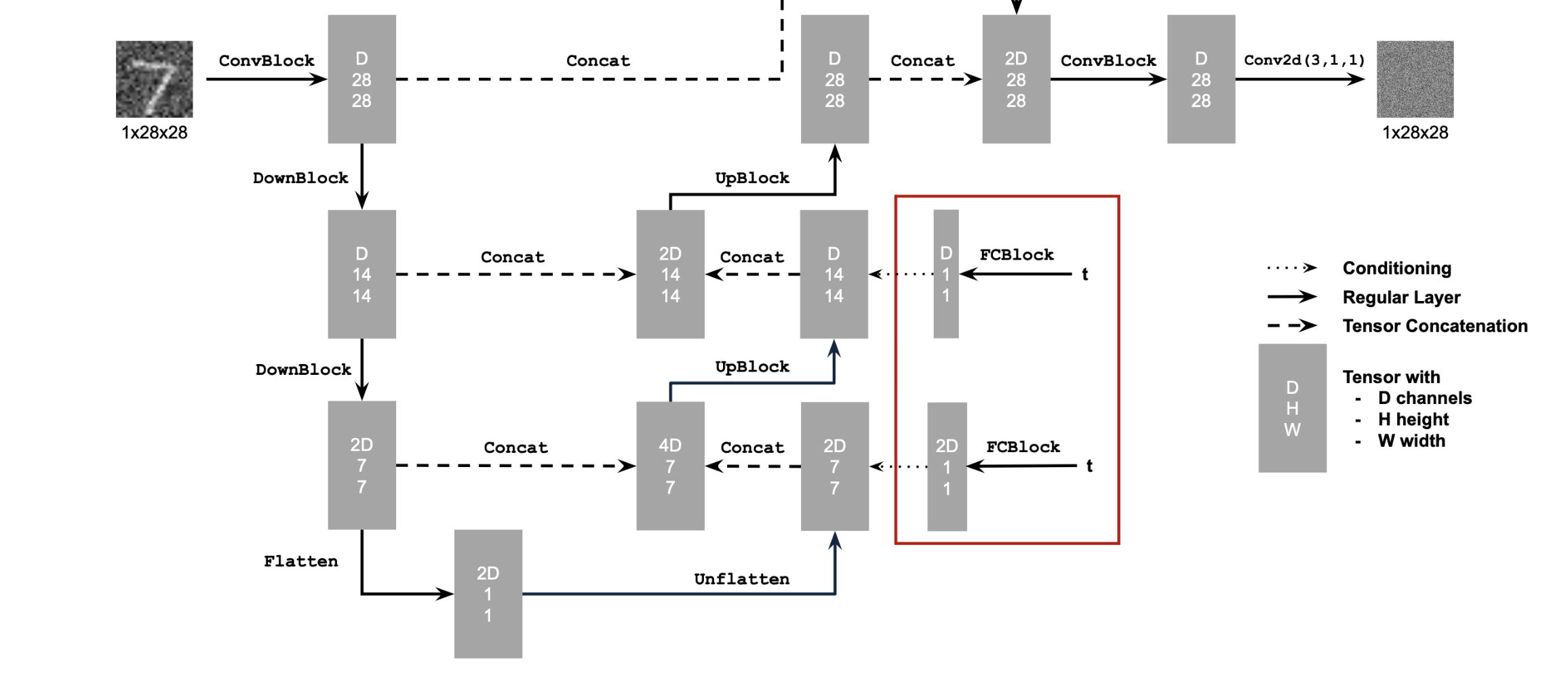
Training the Time Conditioned UNet

Now, we can train our time conditioned UNet by following the below algorithm with the following information: batch size = 128, initial learning rate = 1e-3, optimizer = adam, gamma (lr decay schedule) = 0.1^(1/20), 20 epochs, hidden dimensions = 64

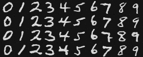
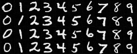
Here are the results:

Epoch 5

Epoch 5

Epoch 20

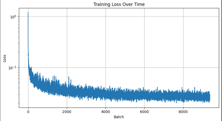
Training Loss Curve

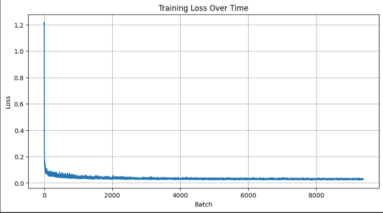
Training Loss Curve

Class Conditioned UNet

The previous samples are generated from pure noise without any labels, that is, they are technically at random. Now, in order to have more control over the generated images, we are going to condition the model on the class labels of the images.

In order to do this, we are going to add a new fully connected layer to our model that takes the class label as input and transforms it into a higher-dimensional representation that can be effectively combined with the image features throughout the network. We are going to one-hot encode the class labels and drop the labelling with probability 0.1 in order to ensure it works without being strictly conditioned on the class labels.

As for the sampling process, it's the same as before, only with the addition o f CFG in order to get better results. We have used the same hyperparameters as before.

Here are the results:

Epoch 5

Epoch 20

Epoch 5

Epoch 20