CS180 Project 4: Image Warping and Mosaicing
Deniz Demirtas
In this project, we will leverage our learnings of image warping from the previous projects and build tools that make you think it's magic.
Before we get started, let's remember more about image warping. Image warping refers to the process of applying a spatial transformation to an image, mapping every pixel in the source image to a new location in the destination image. This operation allows changes in the geometry of an image, including moving, rotating, scaling, or applying a more complex deformation such as perspective adjustments. The transformation can be applied in two ways: forward warp or inverse warp. In a forward warp, pixels from the source image are mapped directly to new positions in the destination image, which can result in gaps if some destination pixels are not assigned a value. In an inverse warp, each pixel in the destination image is mapped back to the source image to determine its value, ensuring complete coverage without missing pixels. The goal of image warping is to modify the image such that it aligns with a different reference plane, corrects distortions, or integrates seamlessly with other images, as in the case of mosaicing or panorama stitching.
Homografies
To calculate a homography matrix (H), we need at least four
pairs of corresponding points between two views of the same planar scene. A
homography is a 3x3 projective transformation matrix that relates the
coordinates of points in one image to those in another image, particularly when both images are
taken from different viewpoints. The homography matrix (H) has eight
degrees of freedom (as it has nine elements, but one is typically fixed for
normalization purposes), allowing it to represent transformations like rotation, translation,
scaling, and perspective effects.
Intuitively, calculating a homography involves understanding the relationship between two images of the same plane but captured from different angles or perspectives. The key idea is that if you can find a set of corresponding points between the images, you can use these points to determine how one image can be warped to match the other. This process is critical in applications such as image mosaicing, where different images need to be aligned to create a seamless panoramic view.
To determine the homography, you first need to identify at least four corresponding points in the two images. I have picked these points manually. Once the points are identified, the homography matrix can be calculated by solving a system of linear equations. This matrix contains information about how the images relate to each other, including any rotations, translations, scalings, and perspective changes.
Since the equations that relate the corresponding points are generally non-linear, we simplify the problem by converting them into a set of linear equations. This process involves cross-multiplying to eliminate the denominators, which allows us to represent the transformation in a linear form. The solution to these linear equations provides the values for the elements of the homography matrix.
The final solution is typically found using a method called Singular Value Decomposition (SVD), which provides a least-squares estimate of the homography matrix. This approach ensures that the solution minimizes the error across all corresponding points, resulting in a transformation that best aligns the two images. By understanding the degrees of freedom involved and the way these transformations are computed, we can appreciate the flexibility of homographies in representing complex changes in perspective and alignment between planar surfaces.
Implementation of Homography Calculation
The computeH function takes two sets of corresponding points, im1_pts
and im2_pts, from two images and calculates the homography matrix H
that maps points from the first image to the second. Here is the function in detail:
def computeH(im1_pts, im2_pts):

                            im1_pts = np.asarray(im1_pts)
                            im2_pts = np.asarray(im2_pts)

                            num_points = im1_pts.shape[0]

                            x1, y1 = im1_pts[:, 0], im1_pts[:, 1]
                            x2, y2 = im2_pts[:, 0], im2_pts[:, 1]

                            # Empty matrix
                            A = np.zeros((2 * num_points, 9))

                            # Fill in the rows of A
                            A[0::2, 0:3] = np.stack([-x1, -y1, -np.ones(num_points)], axis=1)
                            A[0::2, 6:9] = np.stack([x2 * x1, x2 * y1, x2], axis=1)

                            A[1::2, 3:6] = np.stack([-x1, -y1, -np.ones(num_points)], axis=1)
                            A[1::2, 6:9] = np.stack([y2 * x1, y2 * y1, y2], axis=1)

                            U, S, Vt = np.linalg.svd(A)
                            h = Vt[-1, :] / Vt[-1, -1]

                            H = h.reshape((3, 3))

                            return H
Step-by-Step Explanation:
- Matrix A Construction: An empty matrix
Ais created with dimensions(2 * num_points, 9). This matrix stores the coefficients of the linear equations derived from the point correspondences. The homography calculation can be formulated as a linear algebra problem. For each corresponding point pair, we derive two linear equations that represent the mapping between the original and destination images. Specifically, for a point(x, y)in the first image and a corresponding point(x', y')in the second image, we can write down two linear equations involving the unknown homography parameters. The matrixAcollects these coefficients such that we can express the entire system in the formA * h = 0, wherehis the vector containing all nine elements of the homography matrix (flattened). - Filling Matrix A: The matrix
Ais filled with appropriate values based on the point correspondences. Each correspondence pair contributes two rows to the matrix, which encode the relationship between the coordinates in the two images. For each point, we generate two equations to express the transformation: one equation for the x-coordinate and one for the y-coordinate. The entries in these rows contain values derived from the coordinates of the points and include terms for the elements of the homography matrix. By setting up this system, we ultimately aim to solveA * h = 0, which describes how the homography transforms points from the first image to align with the corresponding points in the second image. - Singular Value Decomposition (SVD): The function then performs
SVD on the matrix
Ato solve forh. The vectorhis the last row ofVt, which corresponds to the smallest singular value, providing the best solution for minimizing the error inA * h = 0. - Normalization and Reshape: The resulting vector
his normalized by dividing by its last element to ensure scale consistency. Finally,his reshaped into a3x3matrix to form the homographyH.
This approach ensures that the computed homography H best describes the
transformation between the two sets of corresponding points. Using SVD helps in finding the
least-squares solution, making the homography calculation robust even in the presence of minor
noise or errors in the point correspondences.
Warping The Image
The process of image warping using homographies involves applying the inverse of a homography matrix to an image. This technique is used to transform the perspective of an image so that it aligns with a particular viewpoint or geometry. Typically, the direct application of a homography warps the source image to match the destination plane. However, to accurately map the destination image back to the source or to correct distortions, the inverse of the homography matrix is used. This inverse transformation ensures that each pixel in the output image correctly corresponds to pixels in the input image, based on the geometric projection defined by the homography.
Warping an image through a homography involves computing the dot product of the homography matrix with the pixel coordinates extended into homogenous form. This results in new coordinates that dictate where each pixel of the transformed image will be placed. However, since these new coordinates often do not align perfectly with the discrete pixel grid of the output image, interpolation is necessary to determine the final pixel values. Bilinear interpolation is commonly used in this context; it considers the closest four pixels of the original image to estimate the pixel value at a new position by computing a weighted average, taking into account the distances from each of these four surrounding pixels. This method helps in achieving smoother and more visually appealing transformations.
If you are interested more on that, you can visit my previous projects for more detailed breakdowns of the functions used for the above process.
Where the magic starts
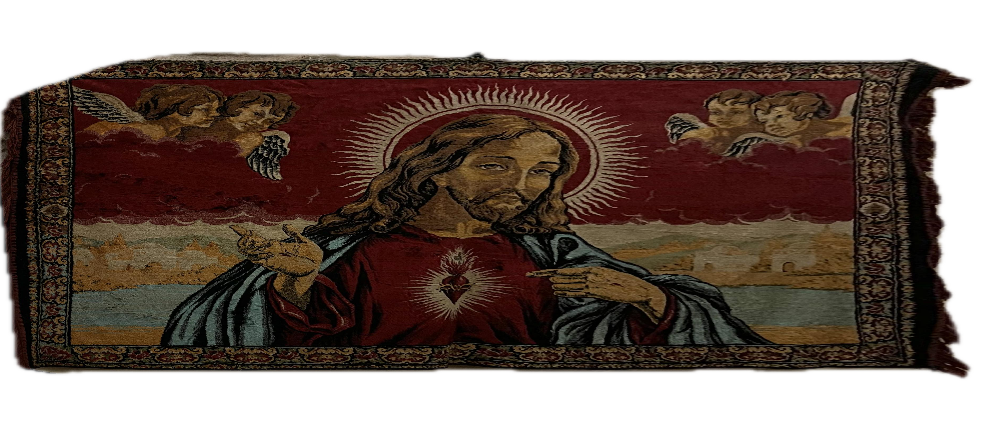
Now, we get to see arguably the most interesting knowledge of my undergraduate education in action as we test the accuracy of our homography calculation and image warping functions. To test this, we are going to generate rectifications of images. This process allows us to visualize certain objects that we select through our correspondences, carrying the visual rays that trace through that object and reconstructing them on another plane to achieve a different perspective of the image. Rectification involves aligning the lines of sight from multiple perspectives into a common plane, typically making the viewing angles perpendicular to the plane. This is achieved mathematically by solving for a homography that maps distorted or tilted planes into a fronto-parallel view, ideal for comparing or measuring physical properties.
With this capability, we are going to generate rectifications of images that mimic the scanning feature of our smartphones by creating perpendicular perspective images of objects photographed from slanted angles. This advanced application enables us to simulate a flatbed scanner effect, providing clear and aligned views of objects as if viewed directly from above, which is invaluable for digital archiving, image analysis, and optical character recognition tasks.
Take a Trip To Mardin, Turkiye with me
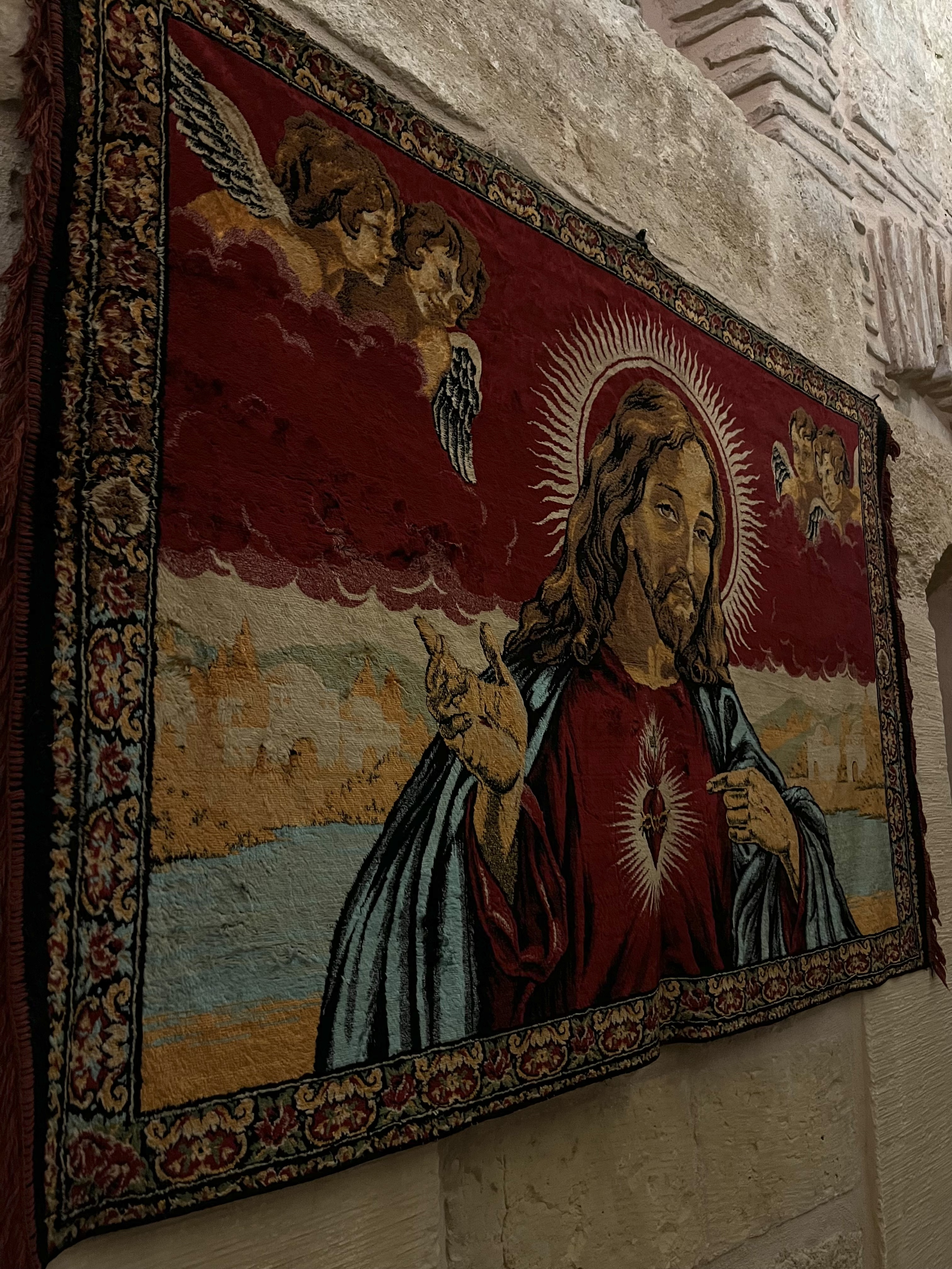
Wall rug from an Assyrian Church in Mardin
Why not take a better look and appreciate it's creation more
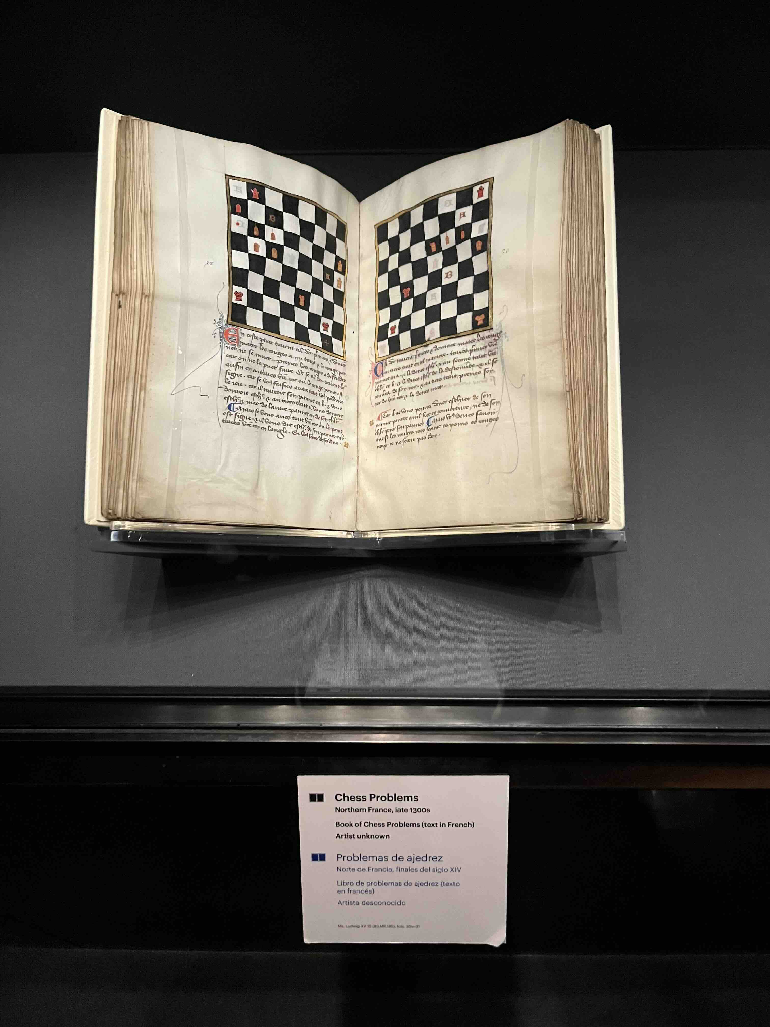
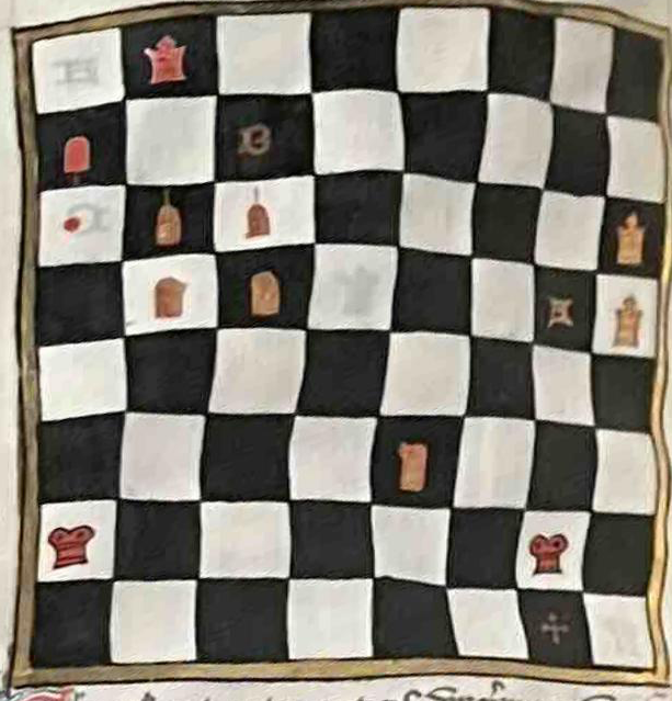
Curious for chess problems from late 1300s?
Amsterdam Naval Museum
Oorlog om winst, winst uit oorlog - War for profit, profit from war
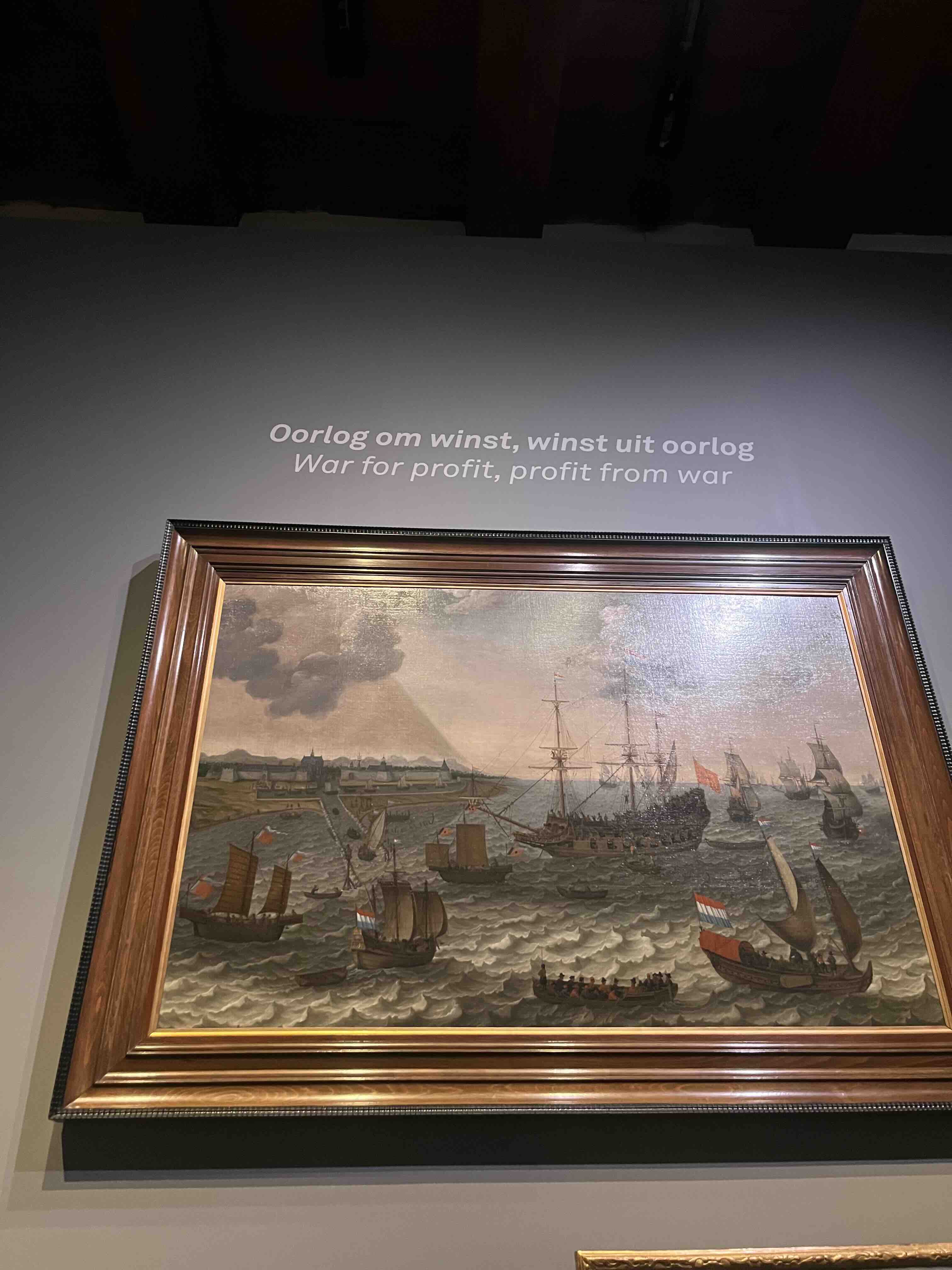
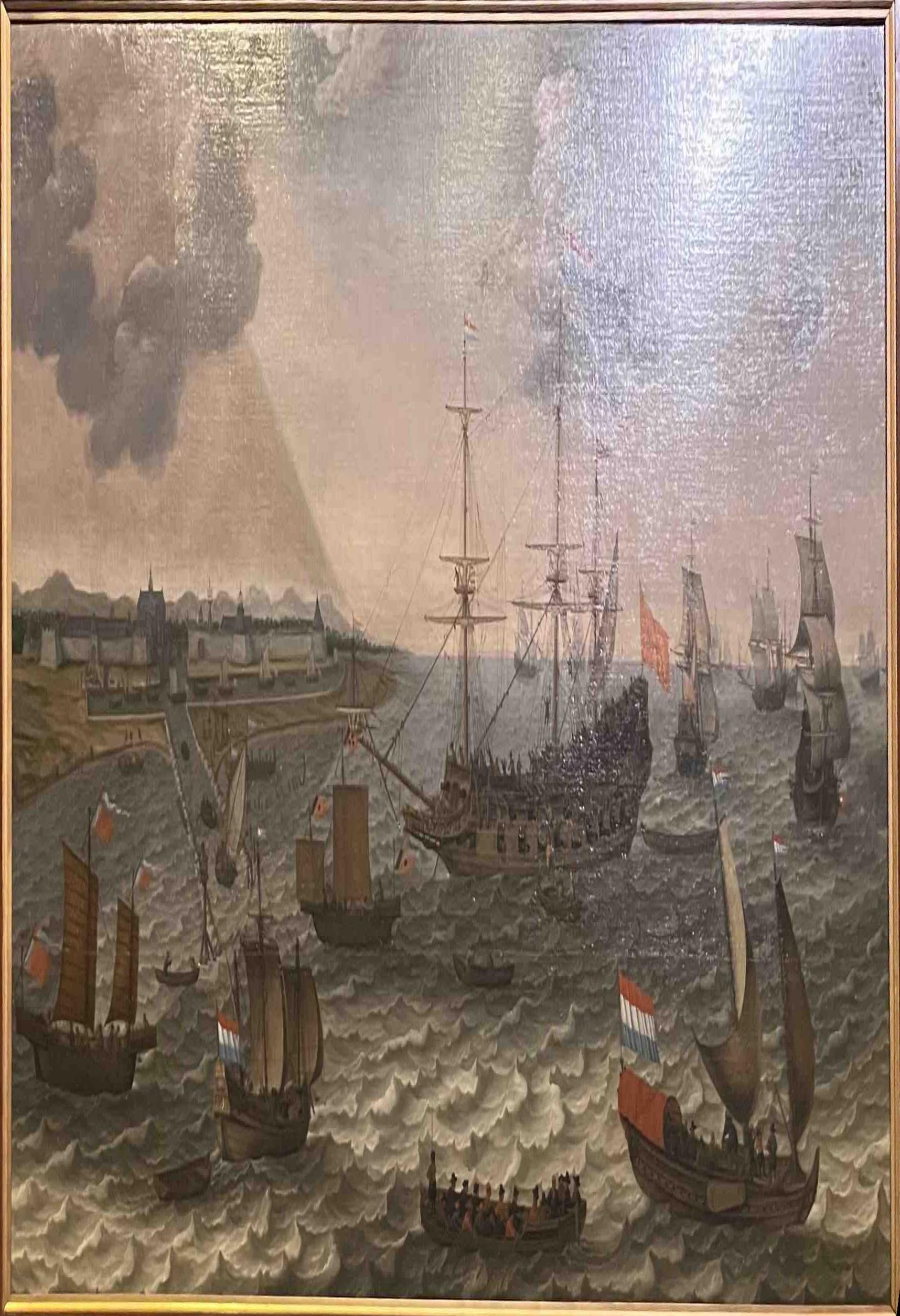
Creating The Image Mosaics: Panorama
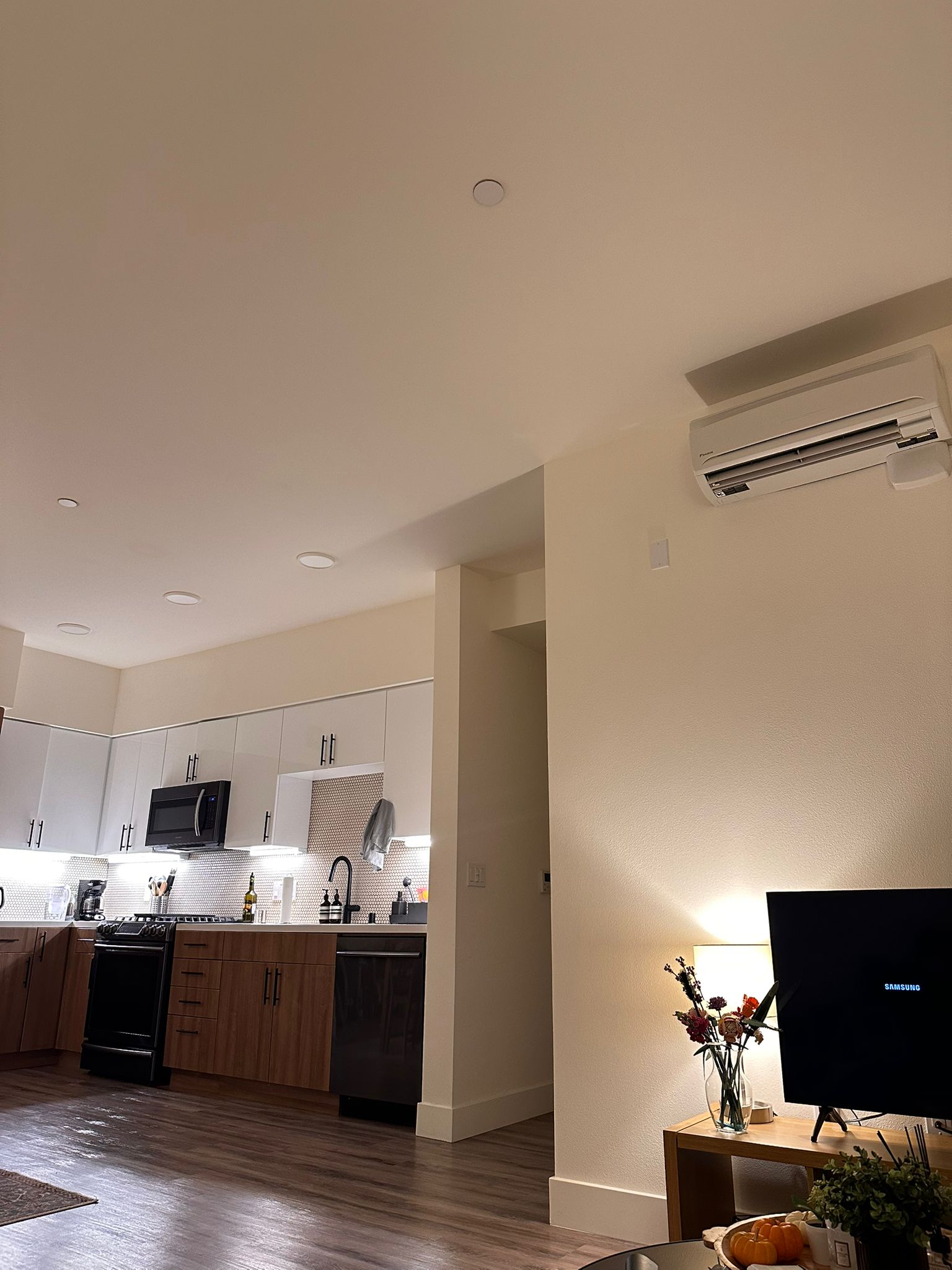
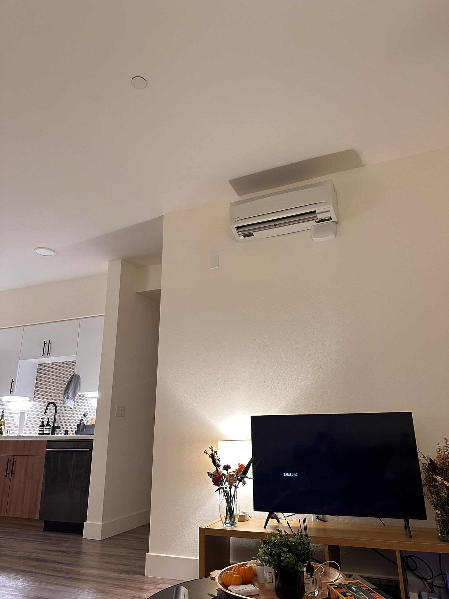
Now, making sure that our functions work correctly so far, we can use them to create image mosaics. Instead of warping the selected object in our initial image to a representation of its geometry in a perpendicular plane, this time we are going to mark the correspondence points between images that have been taken from the same position (with some allowance for slight movements if the images are distant) and use the correspondences to compute the homography that will warp one image onto the geometry of the other. Once warped, the images are blended together to create panoramic pictures.
After we have the warped image, the difference in the workflow starts when we need to create our final canvas for the panorama image to avoid broadcast errors during further operations, since the warped image now has a different shape than the original. We create the final canvas by identifying the corner points of both the warped and the original images and then comparing these points to determine the maximum canvas size required for the mosaic. After that, we apply our warped and original images onto separate canvases to ensure that all subsequent operations are free of broadcast errors.
coords_y, coords_x = np.indices(tower1_image_warped.shape[:2])

                    valid_x_mask = (coords_x >= 0) & (coords_x < canvas1.shape[1])
                    valid_y_mask = (coords_y >= 0) & (coords_y < canvas1.shape[0])

                    valid_mask = valid_x_mask & valid_y_mask
                    non_black_mask = ~np.all(tower1_image_warped == [0, 0, 0], axis=-1)

                    # Combine the valid mask and non-black mask to ensure only valid, non-black pixels are transferred
                    final_mask = valid_mask & non_black_mask

                    # Apply the final mask to place the warped image pixels onto the canvas
                    canvas1[coords_y[final_mask], coords_x[final_mask]] = tower1_image_warped[final_mask]
This code ensures that only the valid pixels from the warped image are placed onto the
canvas.
The coords_y and coords_x arrays represent the pixel coordinates
of
the warped image. The valid_x_mask and valid_y_mask are used to
identify pixels that lie within the bounds of the canvas, while non_black_mask
identifies pixels that are not black (i.e., non-zero values). The final_mask
combines these conditions, ensuring that only valid, non-black pixels are applied to the
final
canvas, preventing any errors or unintended artifacts during the mosaic creation process.
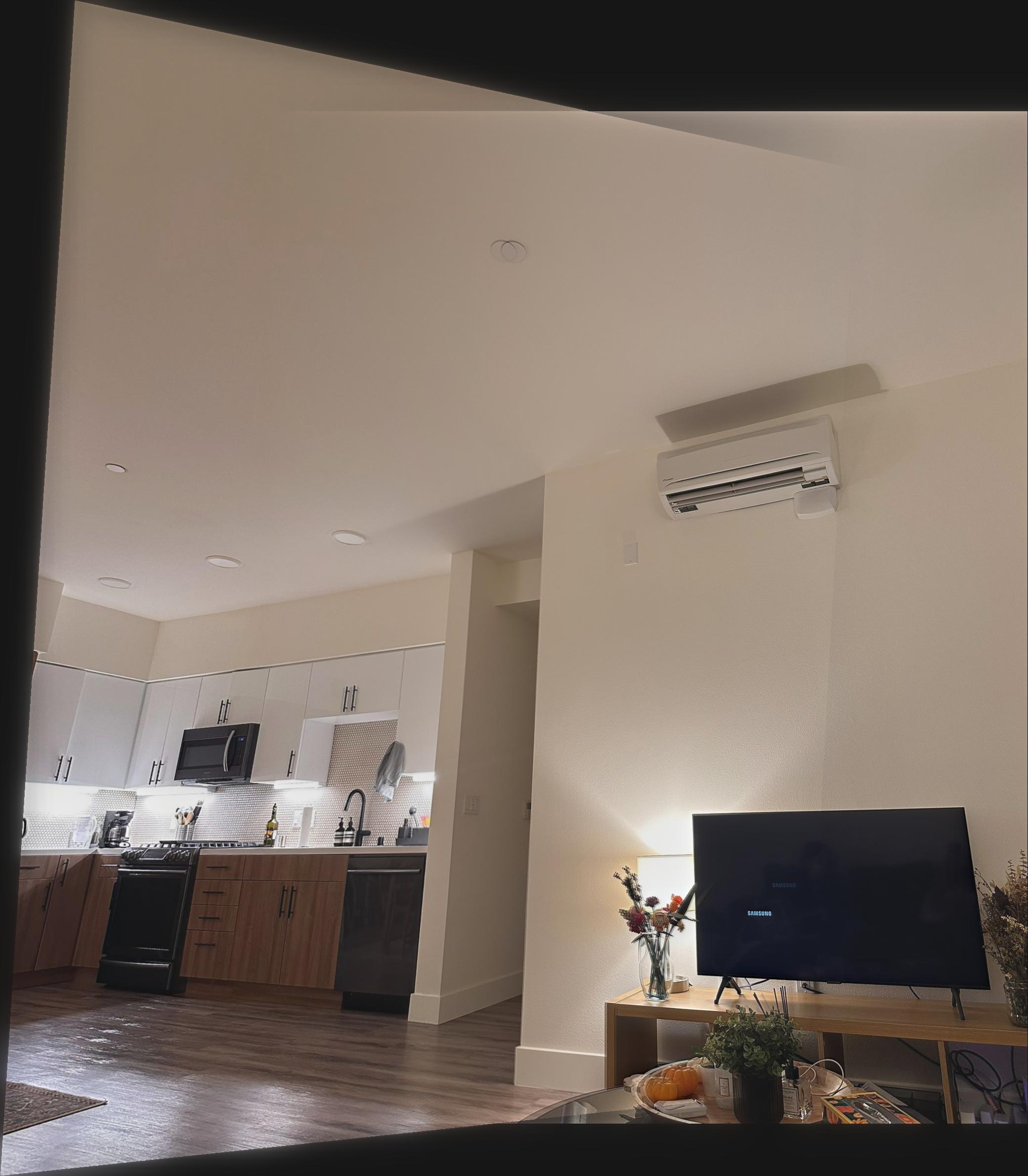
At this point, we can create panoramic pictures with effective overlap if the correspondence points are appropriately selected. However, the seam between the two images will often be noticeable, making the mosaic appear less like a single, unified image. To address this, we use Laplacian blending to create a smooth transition between the images. Unlike simple masking, this requires an automatic and dynamic approach to create a blending mask that adapts to the specific overlap region of the images.
The blending mask is automatically generated by identifying the overlapping regions between the two images and then creating a gradient that smoothly transitions from one image to the other. This gradient ensures that the blending area between the two images is smooth, eliminating sharp edges and visible seams. The blending mask is constructed using distance transforms, which calculate the distance from each pixel in the overlapping area to the boundaries of the overlap. The mask is then refined to ensure smooth blending across the entire overlap, with a focus on maintaining a consistent gradient transition.
Once the blending mask is created, we use it to perform Laplacian blending. The process begins with the construction of Gaussian pyramids for each image, which are formed by iteratively downsampling the images. These Gaussian pyramids are then used to create Laplacian pyramids by subtracting an upsampled version of the next level from the current level, capturing the high-frequency details. We blend the images at each level of the Laplacian pyramid using the Gaussian version of our mask, and finally, we reconstruct the blended image by combining all the levels. This results in a seamlessly blended panorama, where the transitions between the images are smooth and natural.
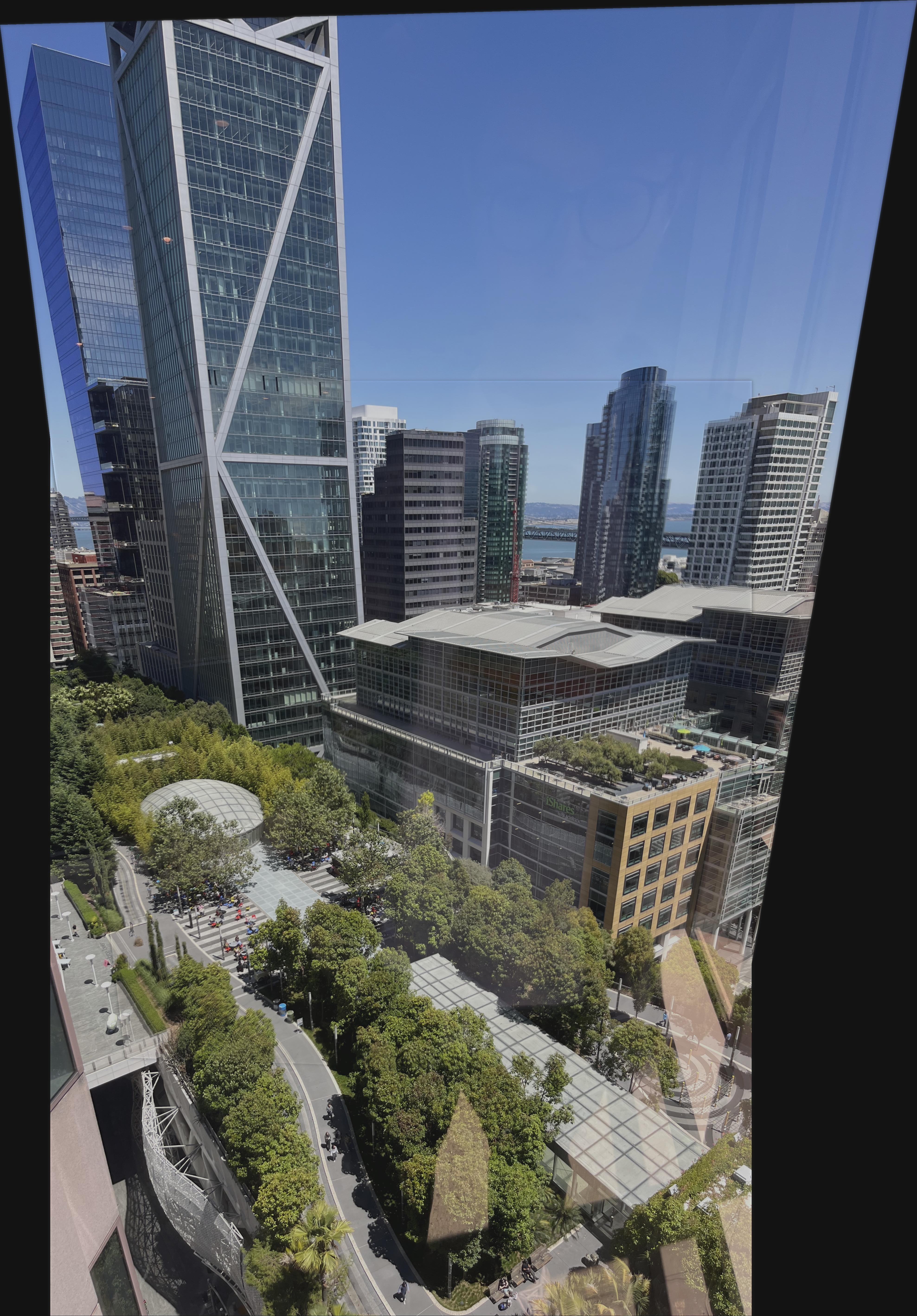
Have a look at the view with me
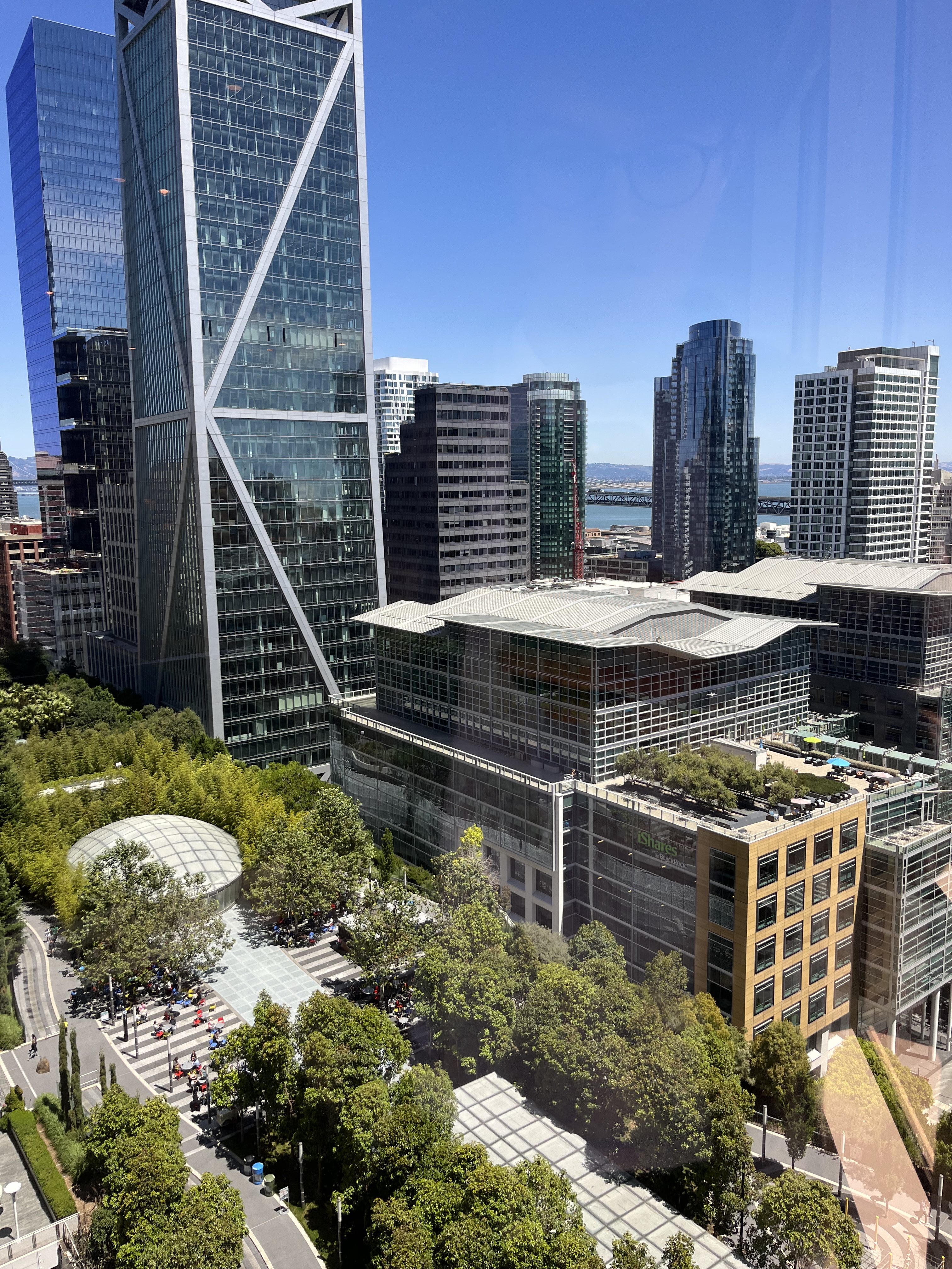
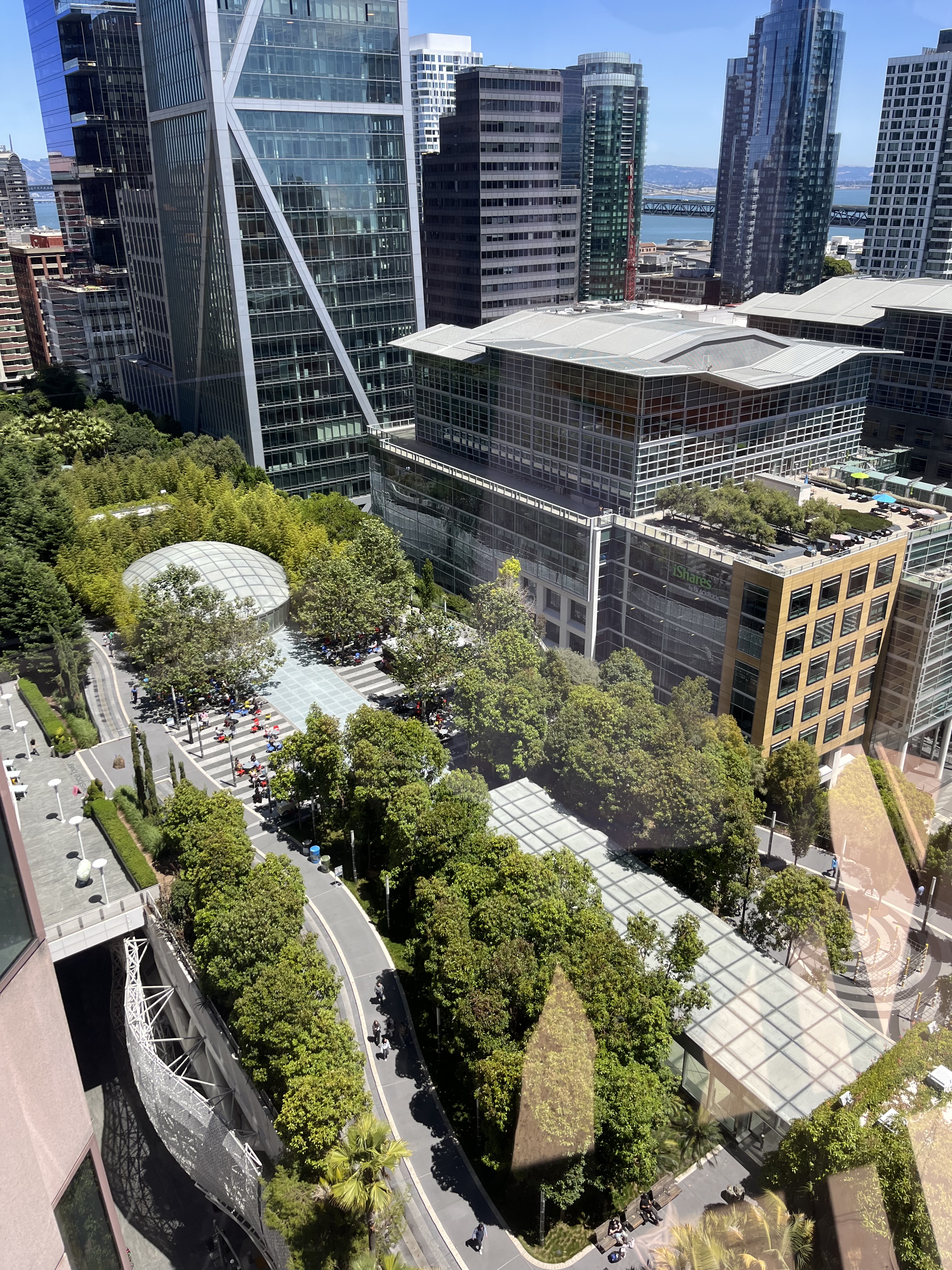
Panorama!
Couch view
Panorama!
FEATURE MATCHING for AUTOSTITCHING
Harris Corner Detection
While manual selection of correspondence points can work, it's prone to errors and incredibly time-consuming—even a few pixels of misalignment could necessitate starting over. As any sane computer scientist would do, we naturally seek to automate and optimize this process. To achieve this, we implemented the methodology described in the paper "Multi-Image Matching using Multi-Scale Oriented Patches" by Brown et al. This approach provides a robust and automated solution for feature detection and matching.
The first step in automating feature selection is implementing a reliable method for corner detection in images. Following the paper's methodology, we utilized the Harris Corner Detector.
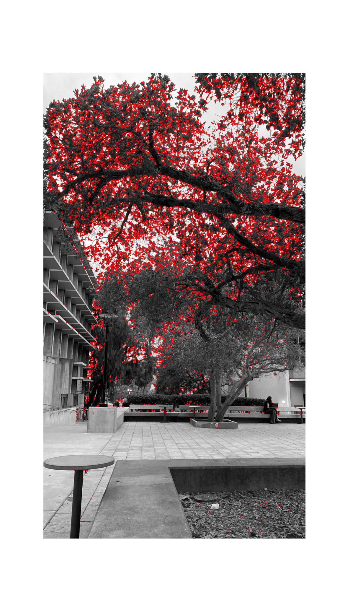
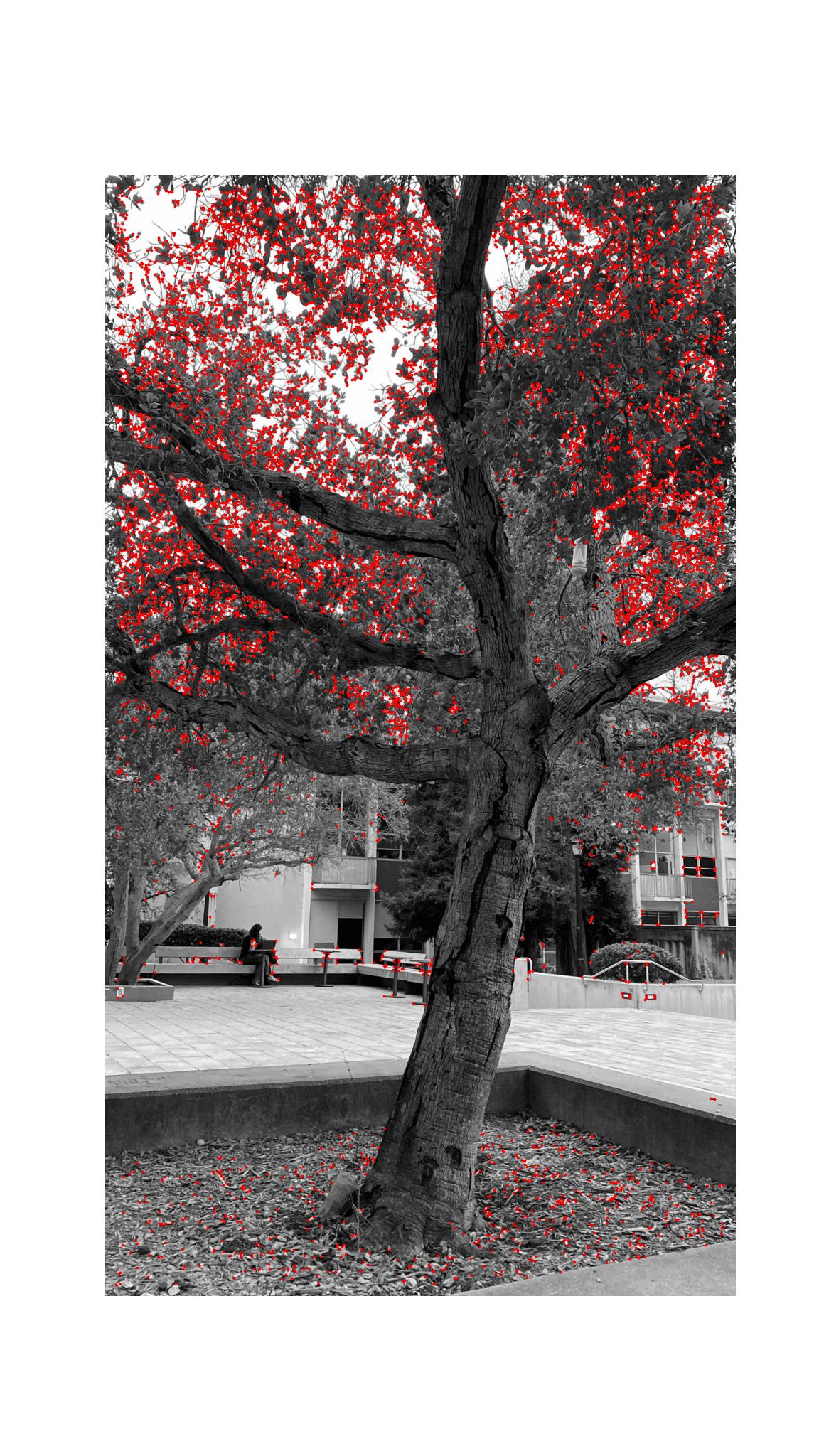
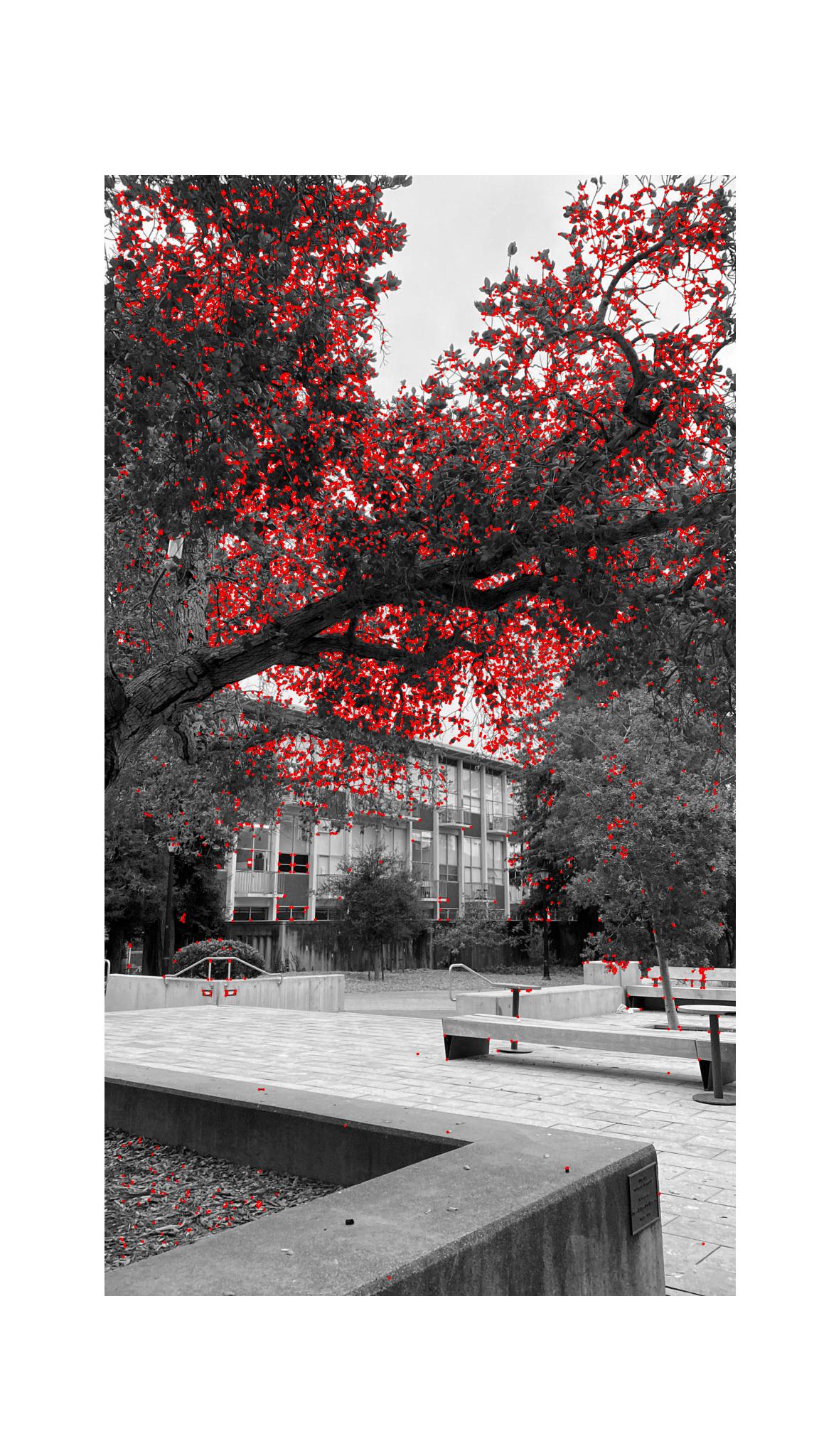
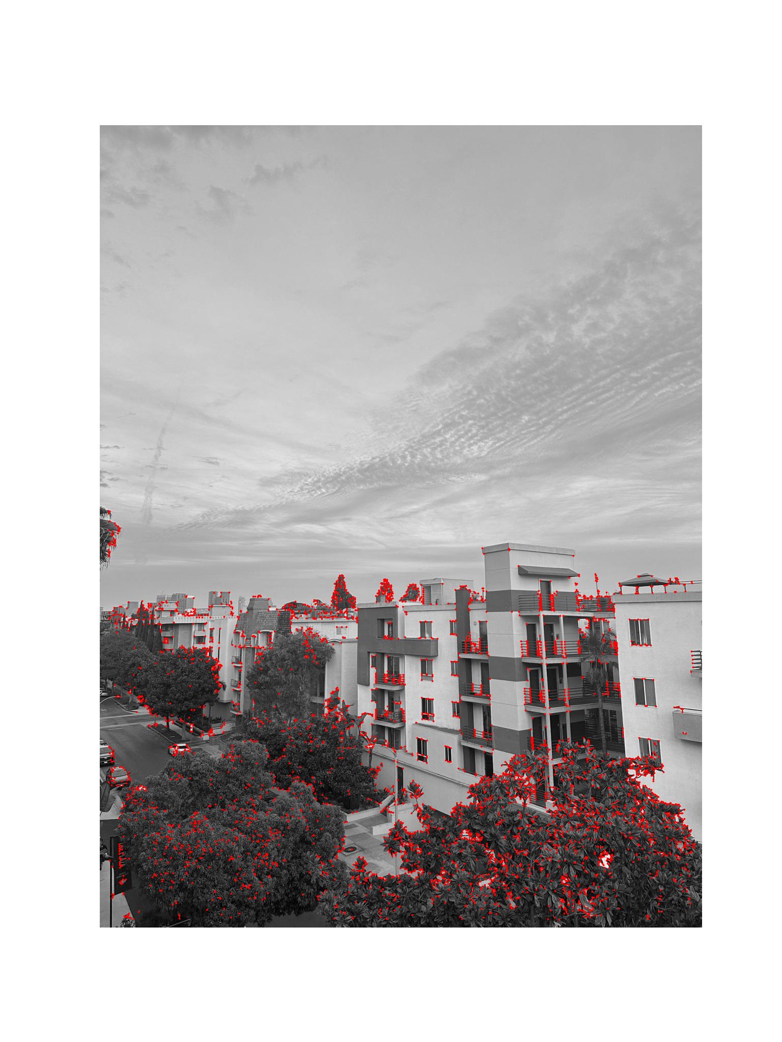
The Harris Corner Detector operates on a fundamental principle: analyzing intensity changes within a small window as it moves across the image. In flat regions, sliding this window in any direction results in minimal intensity changes. Along edges, moving the window perpendicular to the edge direction causes significant changes, while moving parallel to the edge produces little change. At corners, moving the window in any direction results in substantial intensity changes, making corners distinctly identifiable.
Mathematically, the Harris Corner Detector computes the structure tensor matrix M:
where Ix and Iy represent image gradients in x and y directions, and Σw denotes summation over a Gaussian window.
The detector then evaluates each point using the Harris corner response function:
This response function R characterizes different image features:
- R > 0: Indicates a corner region, where high eigenvalues reflect significant intensity changes in all directions
- R < 0: Suggests an edge, where one eigenvalue is significantly larger than the other, indicating directional change
- R ≈ 0: Represents a flat region, where both eigenvalues are small, indicating minimal intensity changes
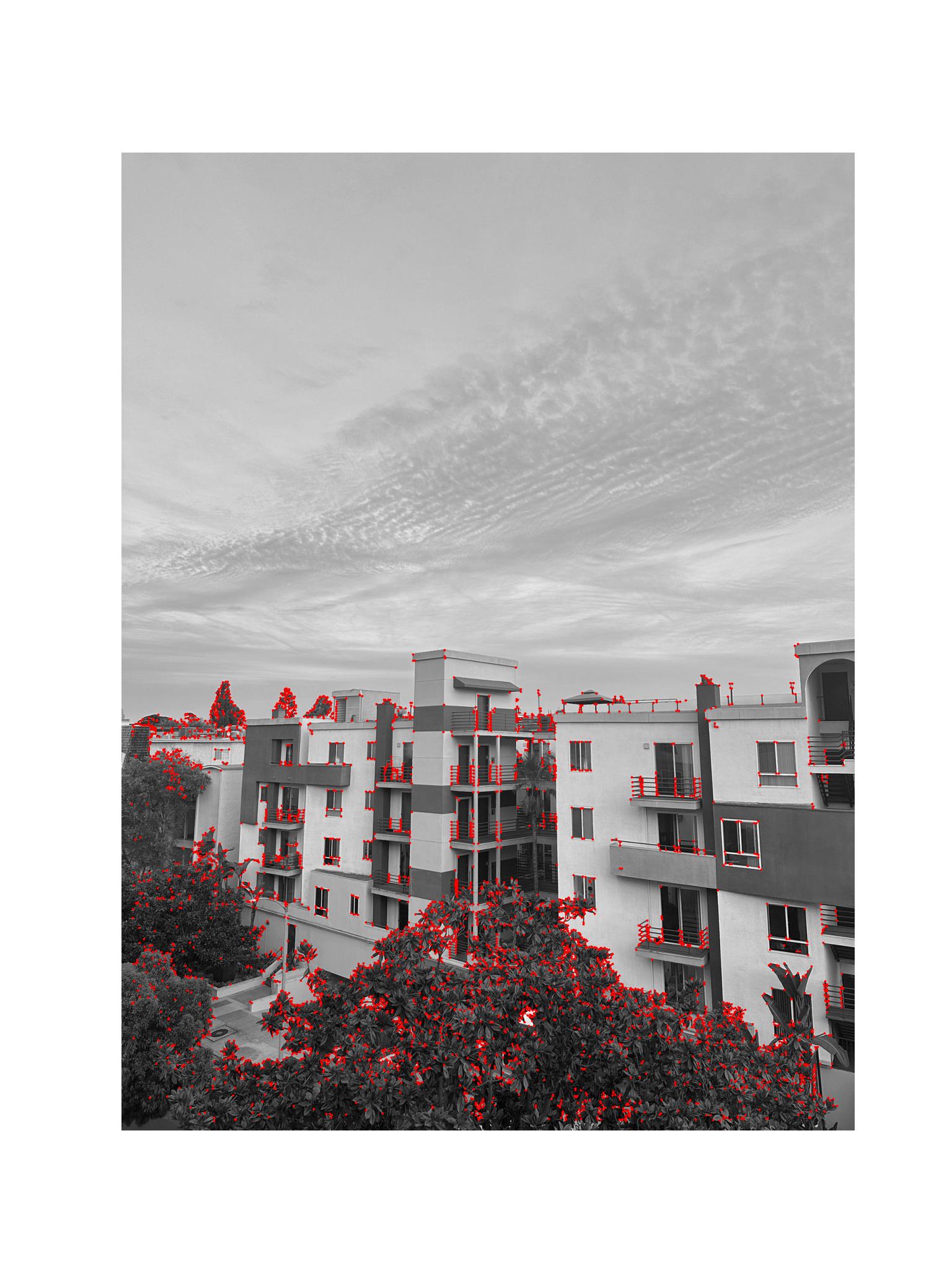
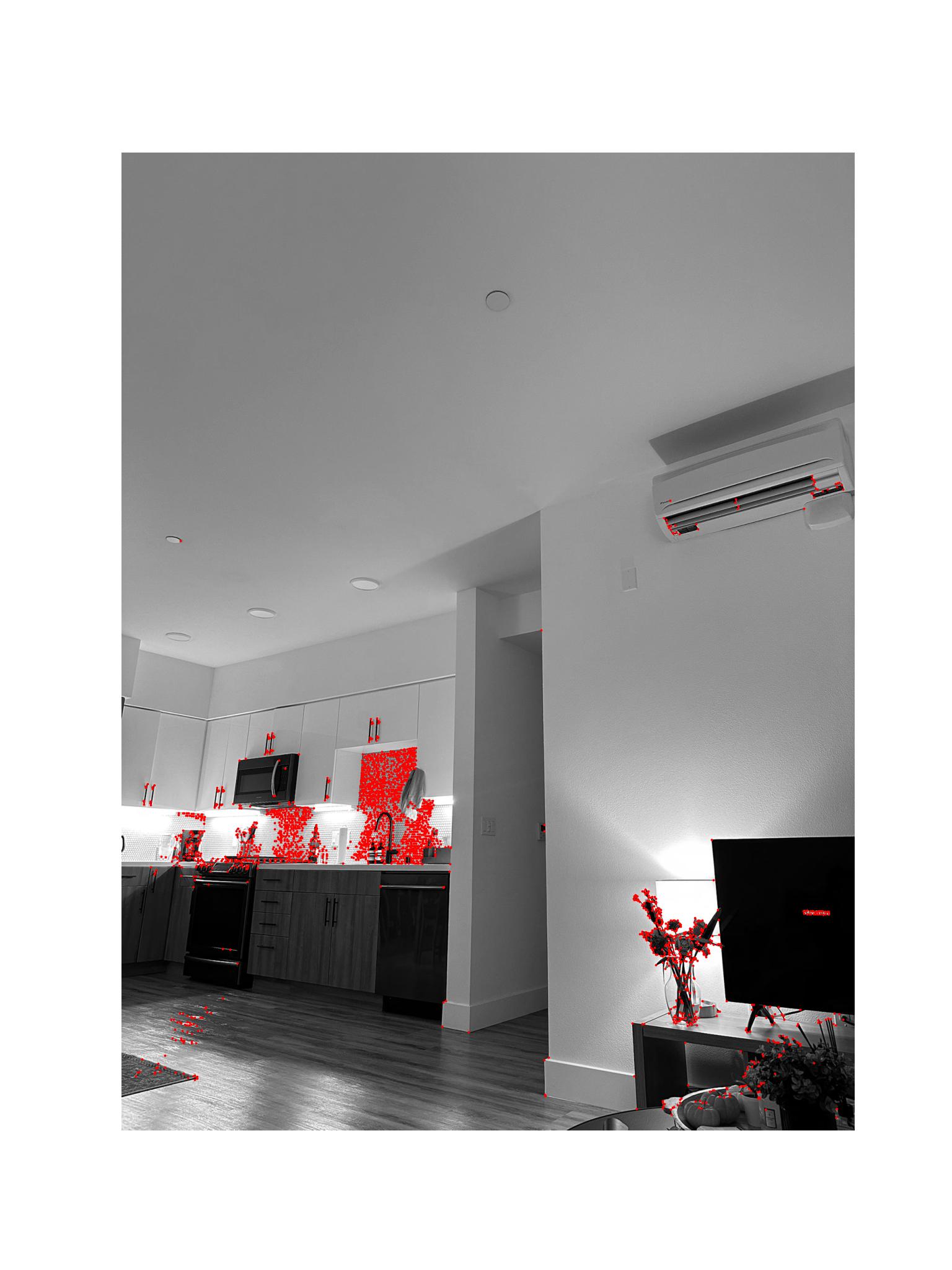
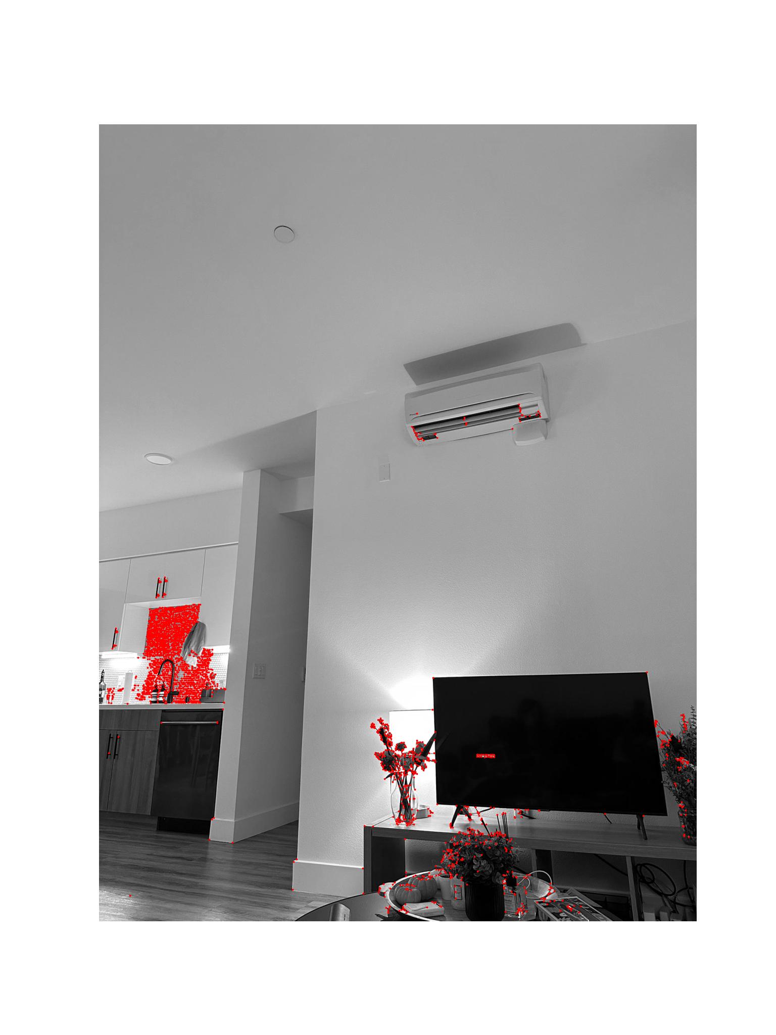
Here are some results from the Harris Corner detector:

Adaptive Non-Maximal Suppression
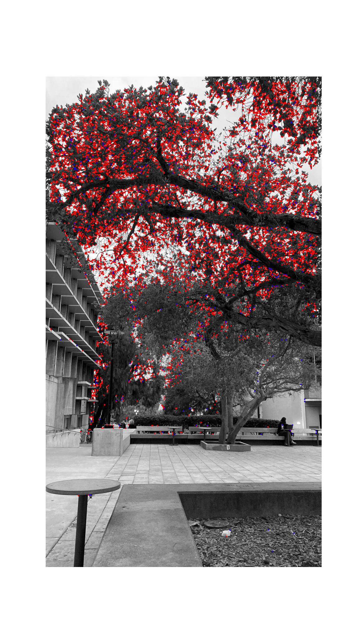
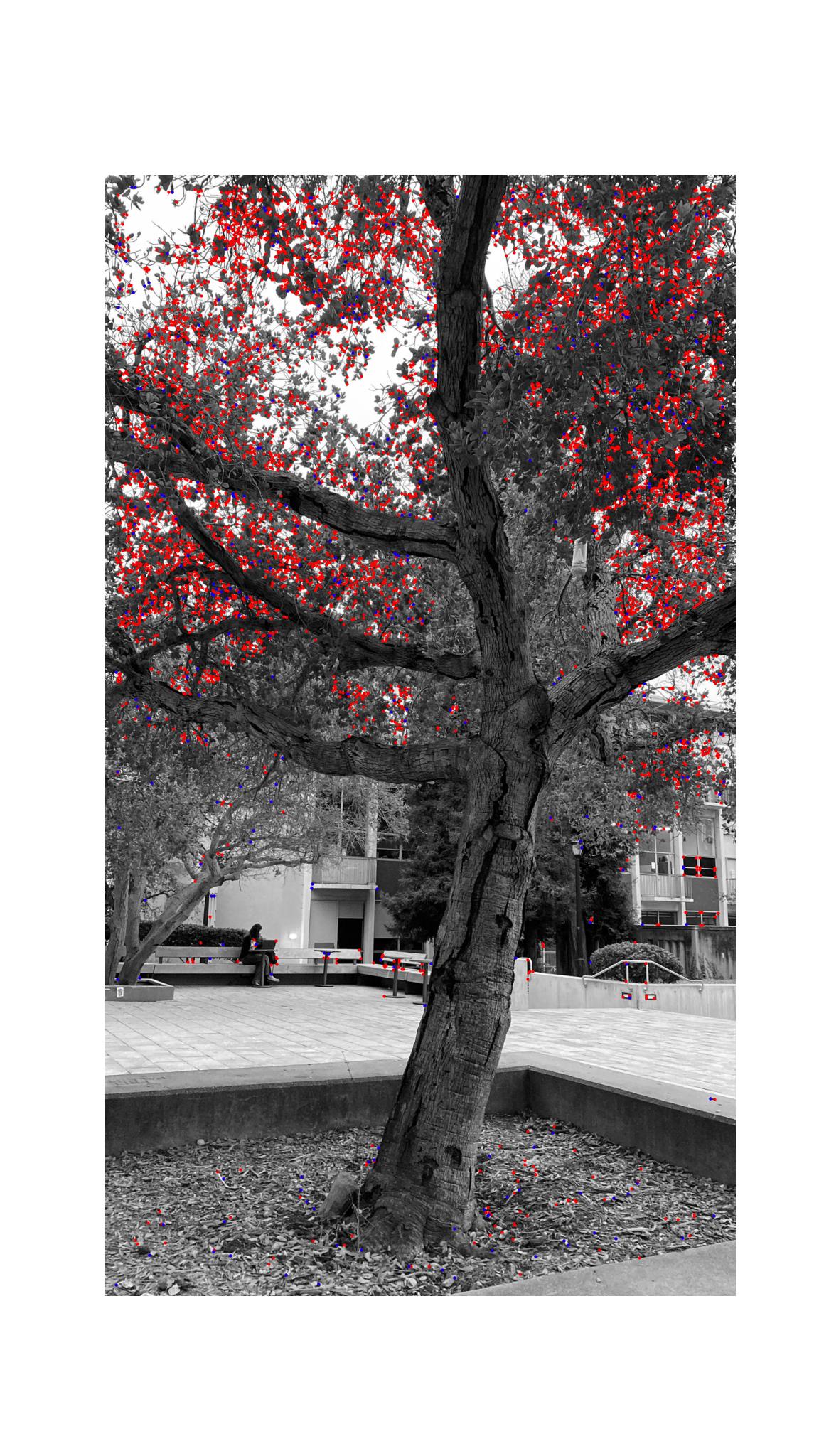
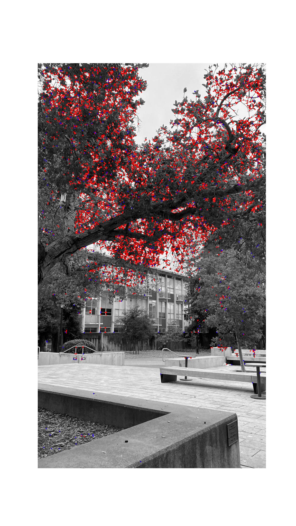
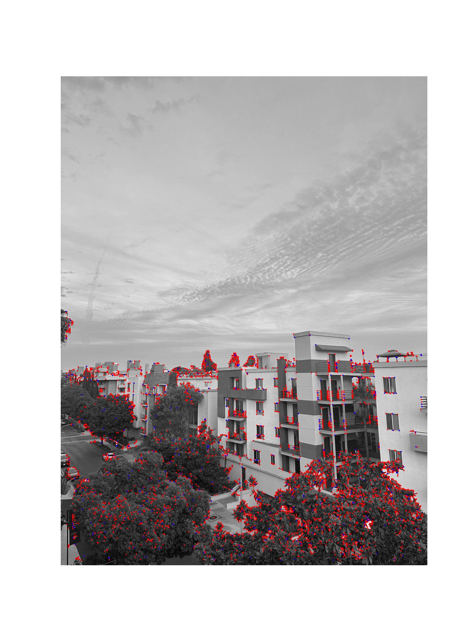
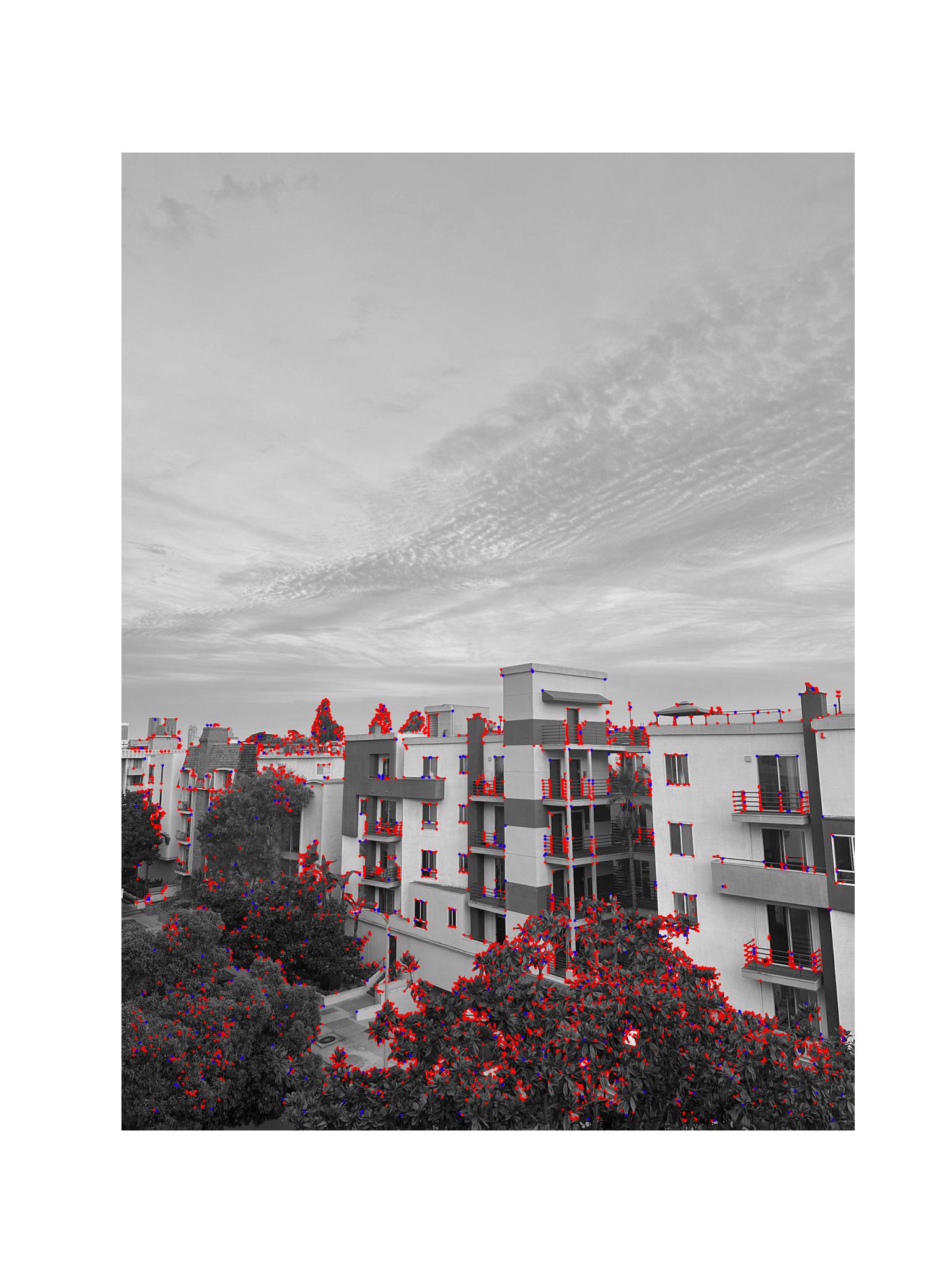
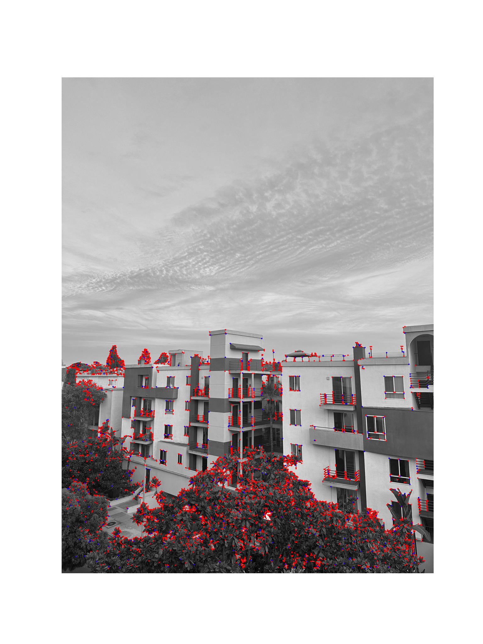
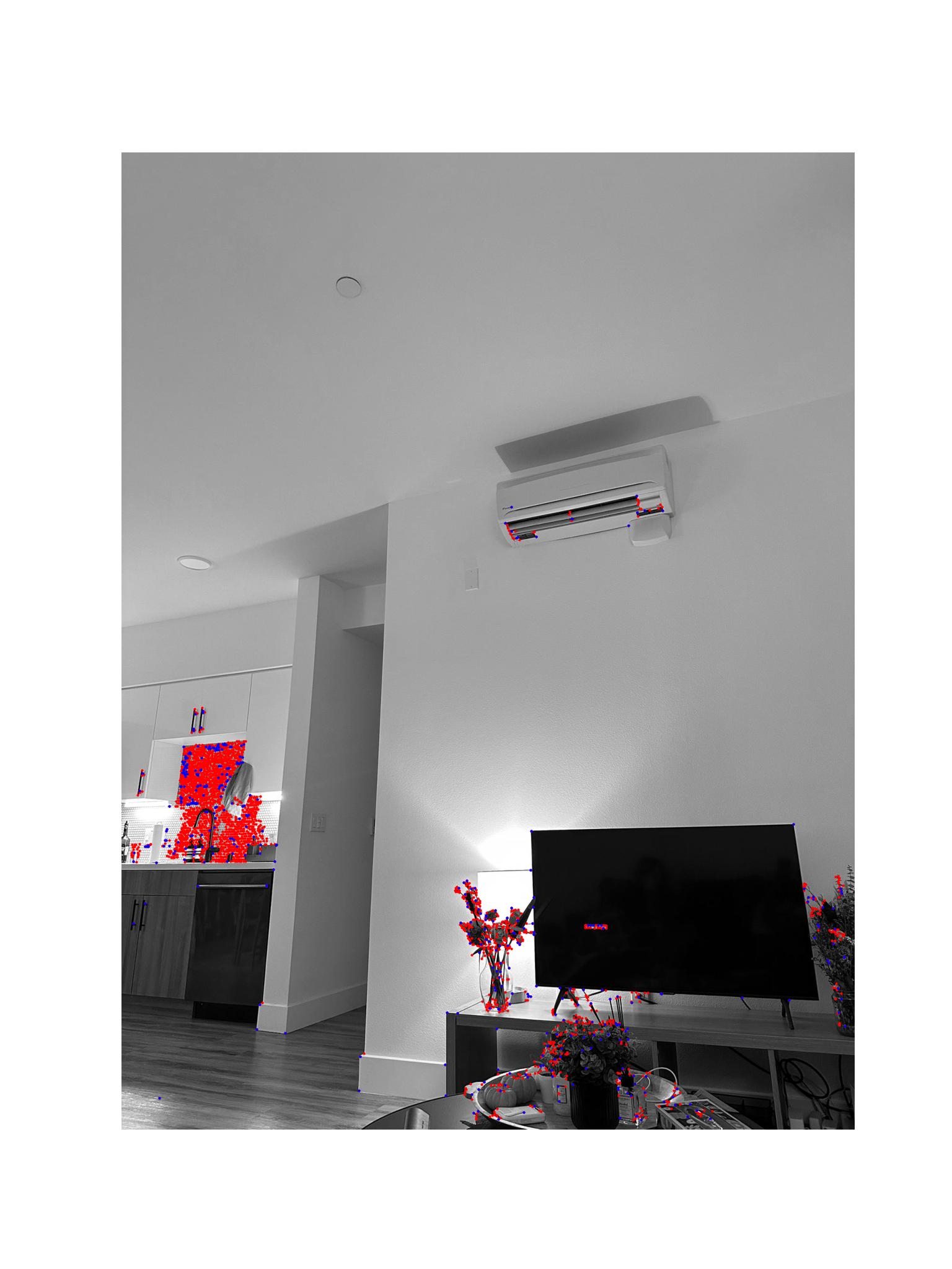
Now that we have automated our corner detection, great news! We no longer have to deal with manually selecting correspondences. However, it's a bit too early to celebrate completely. If you notice, we have no direct control over where the detected corners are located in the image. We can only provide the Harris Corner detection algorithm with a threshold to determine which points qualify as corners, but we can't control the regions from which they are chosen or their distribution. As you may recall from the lecture, the key to a good warp is to have well-distributed correspondences. We need to address this to improve our results.
We are going to achieve this through Non-Maximal Suppression (ANMS), which can be thought of as a way to ensure that we pick corners that are spread out as evenly as possible from the set of all detected corners.
The underlying mathematical intuition is as follows: we first sort every detected corner by its strength. Then, we assign an initial suppressing radius of infinity to each corner, and start iterating from the strongest to the weakest corner. The suppressing radius represents the area within which a given corner is considered the strongest—meaning, within this radius, only that corner will be selected. As we iterate, for each corner, we look at its neighboring corners within its current suppressing radius. If a stronger corner is found within this radius, we update the radius to be the distance to the stronger corner. To efficiently access neighboring corners, I used a kd-tree, which helps find neighbors within the given radius quickly.
This approach ensures that the strongest corners are selected in a way that maximizes their spatial separation. It may result in selecting slightly weaker corners compared to a purely strength-based selection, but the suppression radius helps distribute the selected corners more evenly across the image, leading to a better set of correspondences for tasks like image warping.
Let's observe this with comparing the blue (ANMS) corners with the red (Harris) corners.

Extracting Feature Descriptors
Great! Now we can automatically generate appropriate correspondences to calculate homographies and create panoramas. However, while we have successfully identified correspondences between images, we still face a challenge: when creating panoramas, we need to determine which correspondence in one image matches the same corner in the other image. Without this matching information, having correspondences alone is not useful. Therefore, we need a method to reliably match these correspondences between images.
To achieve this, we will use feature descriptors. For this project, the feature descriptors are represented by 40x40 pixel patches around each detected corner. After extracting the 40x40 patch, we apply a Gaussian blur to reduce high-frequency noise and then downsample it by selecting every 5th pixel, resulting in an 8x8 patch. This process helps make the descriptors more computationally efficient, reduces sensitivity to noise, and increases invariance to small changes in the image. Finally, we bias-gain normalize the descriptors by adjusting the mean to zero and the standard deviation to one, making them invariant to changes in illumination and contrast across different images.
Here are couple examples - in the same order with the images in previous parts


Feature Matching
Now, we still don't have the matchings of our features. However, we now have a metric that we can use to compare the features with each other and match them.
For the matching algorithm, I have designed an object-oriented approach to maintain a clear and organized codebase.
                                    class DescriptorMatcher:

                                        def __init__(self, descriptors_dict):

                                            self.descriptors_dict = descriptors_dict
                                            self.descriptors = np.array(list(descriptors_dict.values()))
                                            self.coordinates = list(descriptors_dict.keys())
                                            self.num_descriptors = len(self.descriptors)
                            def match_features(self, other_matcher, threshold=0.5):
                            matches = {}

                            for i, query_descriptor in self.descriptors_dict.items():

                                # Find the 1st and 2nd nearest neighbors in the other matcher's descriptors
                                nn_1_idx, nn_1_distance = other_matcher.find_nn(query_descriptor, k=1)
                                _, nn_2_distance = other_matcher.find_nn(query_descriptor, k=2)

                                # Calculate the 1-NN/2-NN ratio
                                nn_ratio = nn_1_distance / nn_2_distance

                                # Store the match if the ratio is below the threshold (indicating a good match)
                                if nn_ratio < threshold:
                                    matches[self.coordinates[i]] = other_matcher.coordinates[nn_1_idx]

                            return matches
                            def find_nn(self, query_descriptor, k=1):

                            query_descriptor_flat = query_descriptor.flatten()

                            # Flatten each descriptor in self.descriptors to create a list of 1D descriptors
                            descriptors_flat = np.array([descriptor.flatten() for descriptor in self.descriptors])

                            # Compute the distance matrix between the query descriptor and all stored descriptors
                            distances = distance_matrix([query_descriptor_flat], descriptors_flat)[0]

                            # Get the indices of sorted distances (in ascending order)
                            sorted_indices = np.argsort(distances)

                            # Find the k-th nearest neighbor
                            kth_nn_idx = sorted_indices[k - 1]
                            kth_nn_distance = distances[kth_nn_idx]

                            return kth_nn_idx, kth_nn_distance
Creating Panoramas: 4-point RANSAC (Random Sample Consensus)
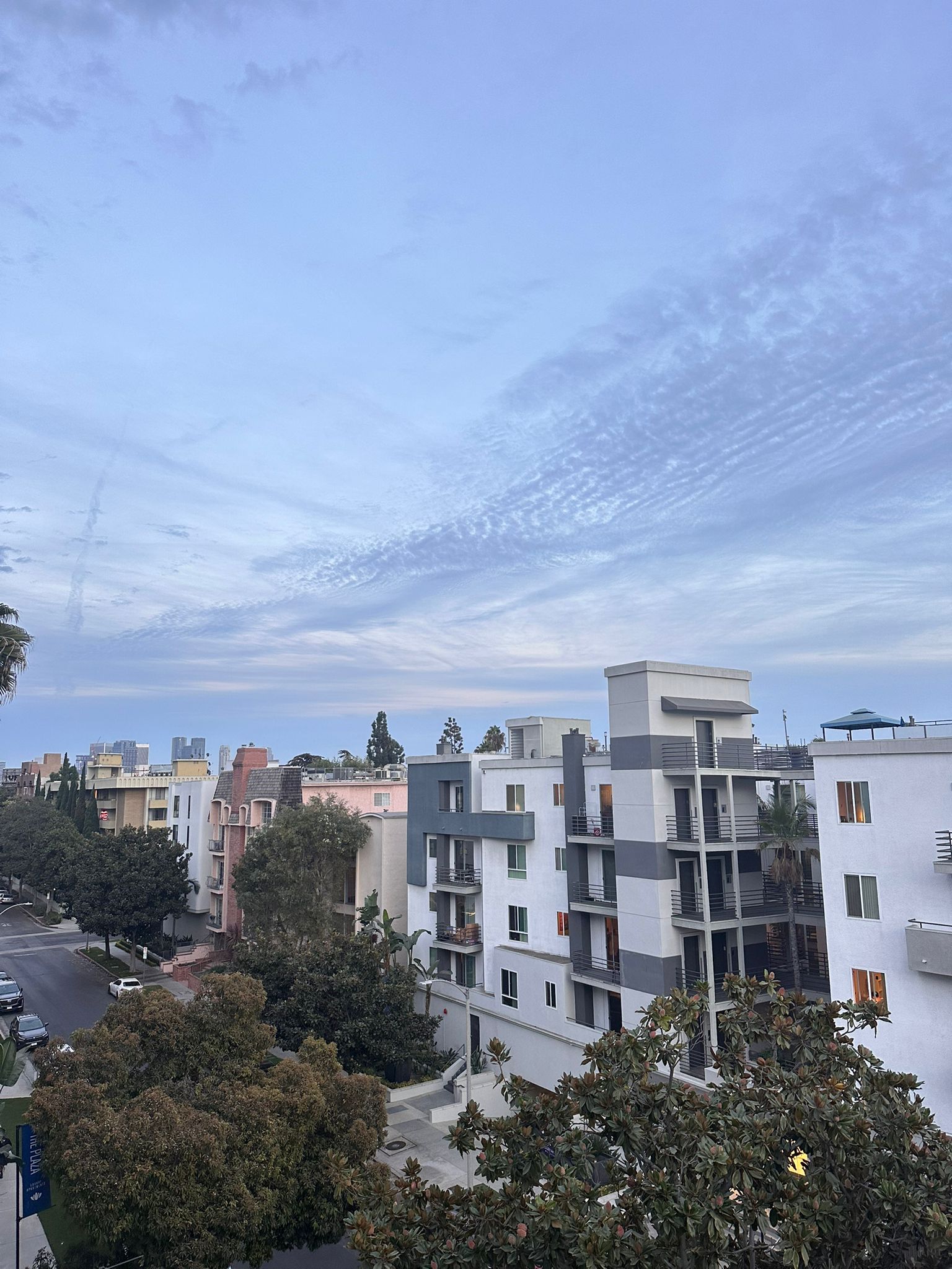
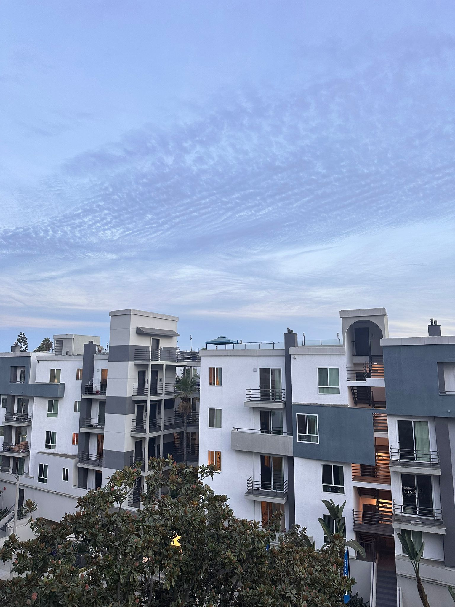
Now that we have matched our features, we can generate the homographies and warp our images to create panoramas. However, instead of generating a homography using all of our points directly, we prefer to use RANSAC to ensure the result is robust. RANSAC helps us gather a subset of inlier points by iteratively selecting a random subset of 4 points, calculating a homography, and then checking how well the warped points align with their correspondences. This process is repeated for a specified number of iterations. If the warped point error is below our threshold, we consider it an inlier. After completing all iterations, we use the inliers to run a least-squares estimate to generate the final homography. This ensures that only the best matching points are used for homography creation, resulting in a more accurate and reliable transformation.
The blending of the images after generating the final homography with RANSAC and warping them is similar to the approach used in the first part of the project. We use Gaussian blending to merge the images, creating a blending mask by first identifying the non-background regions. We then calculate the overlap mask to determine where the images overlap, use a distance transform to determine each pixel's distance from the boundary, and finally smooth the blending boundary using a continuous gradient to achieve a seamless transition.
Automatic Panoramas!
View From a LA Balcony - p1
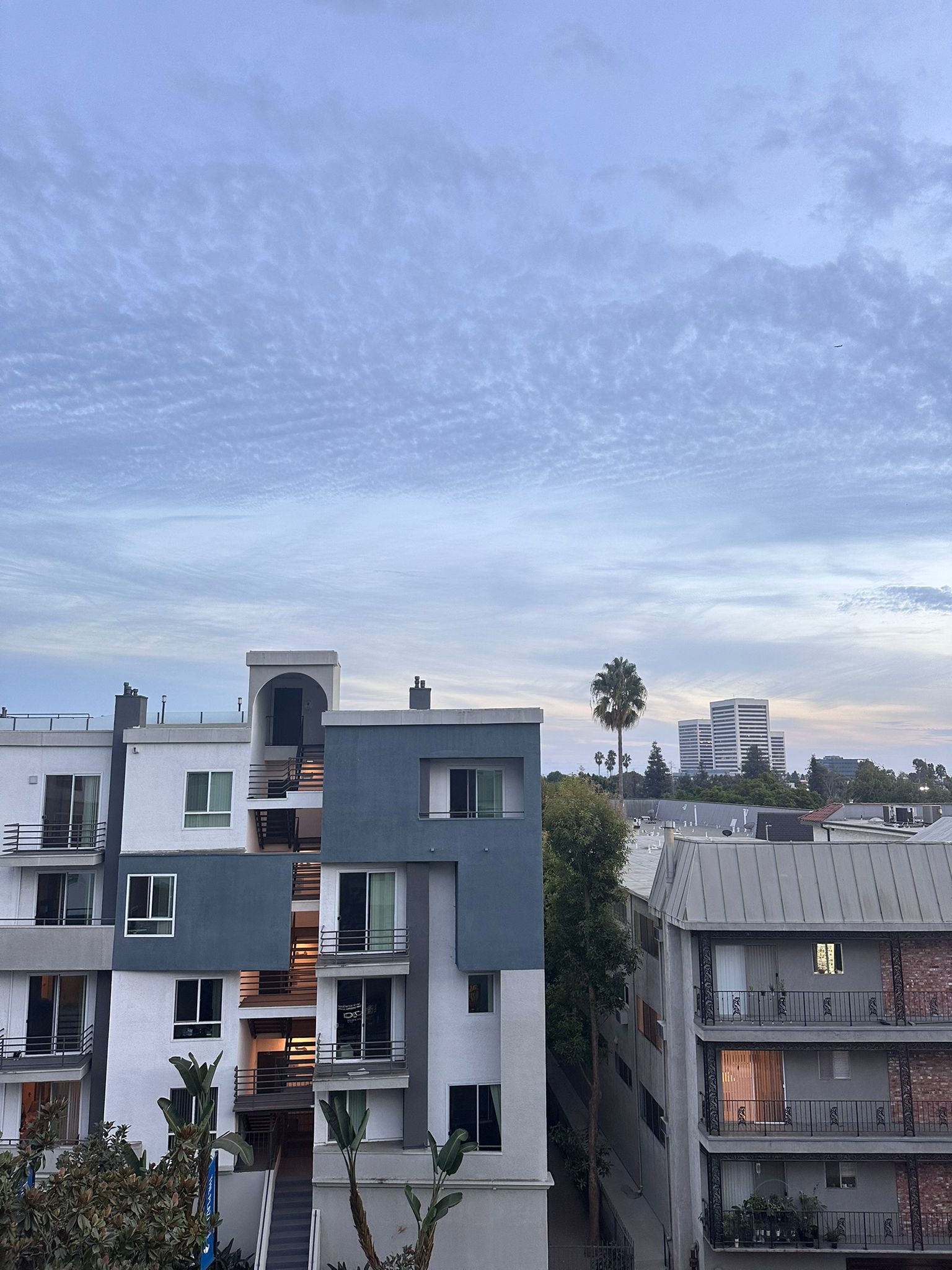
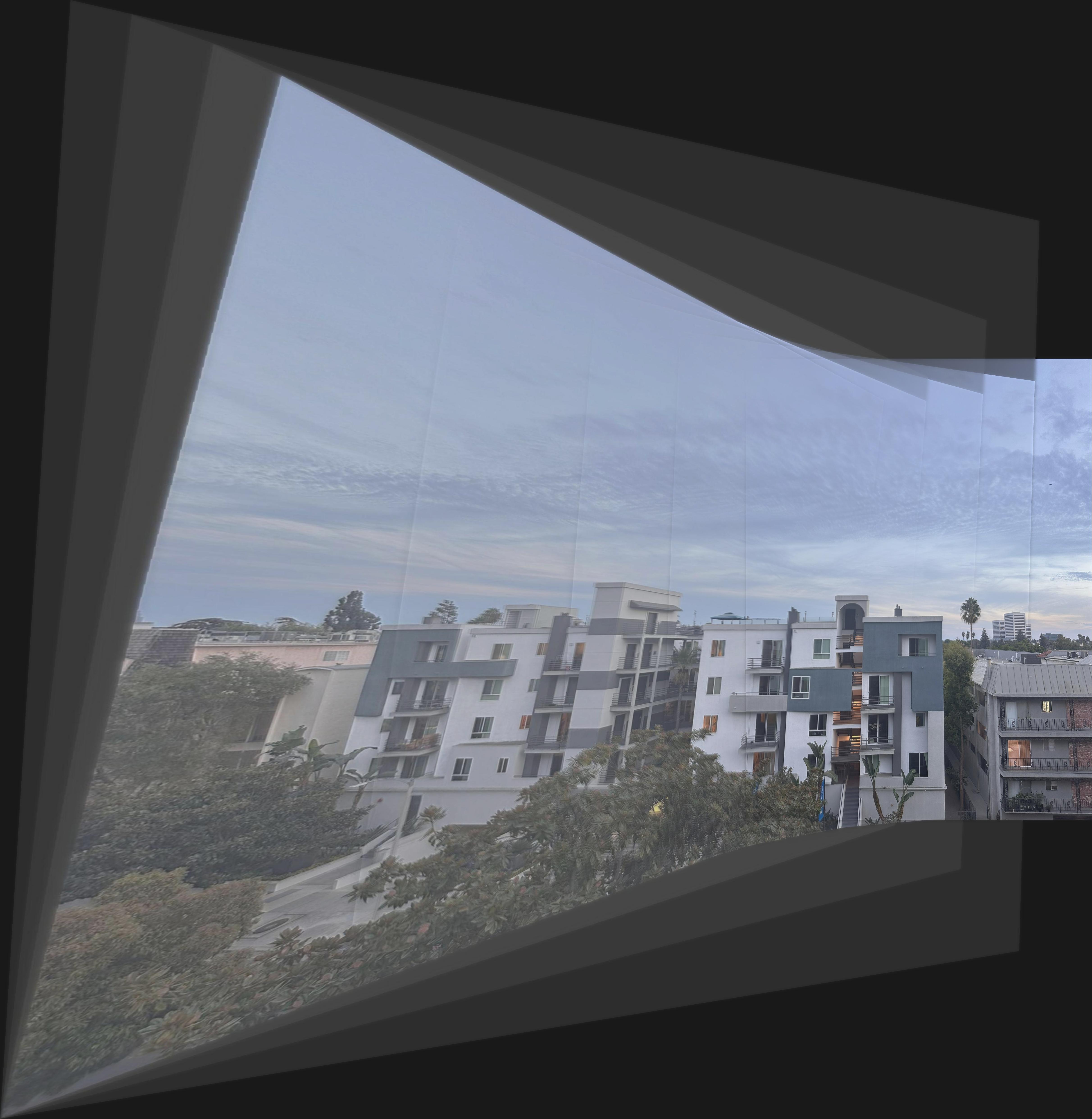
Zoom out with (CMD-) after clicking on the image
View From a LA Balcony - p2
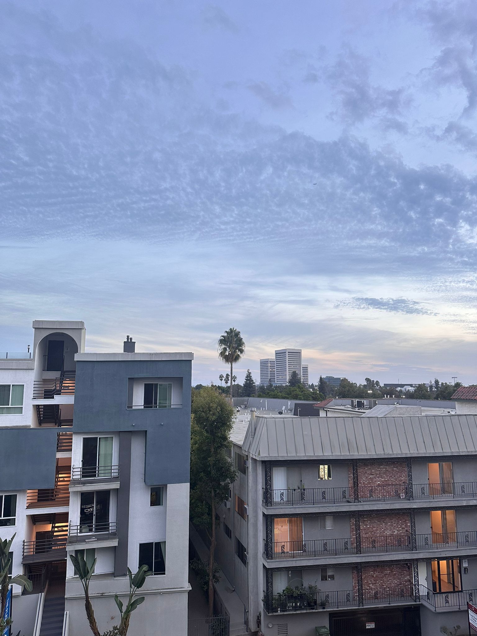
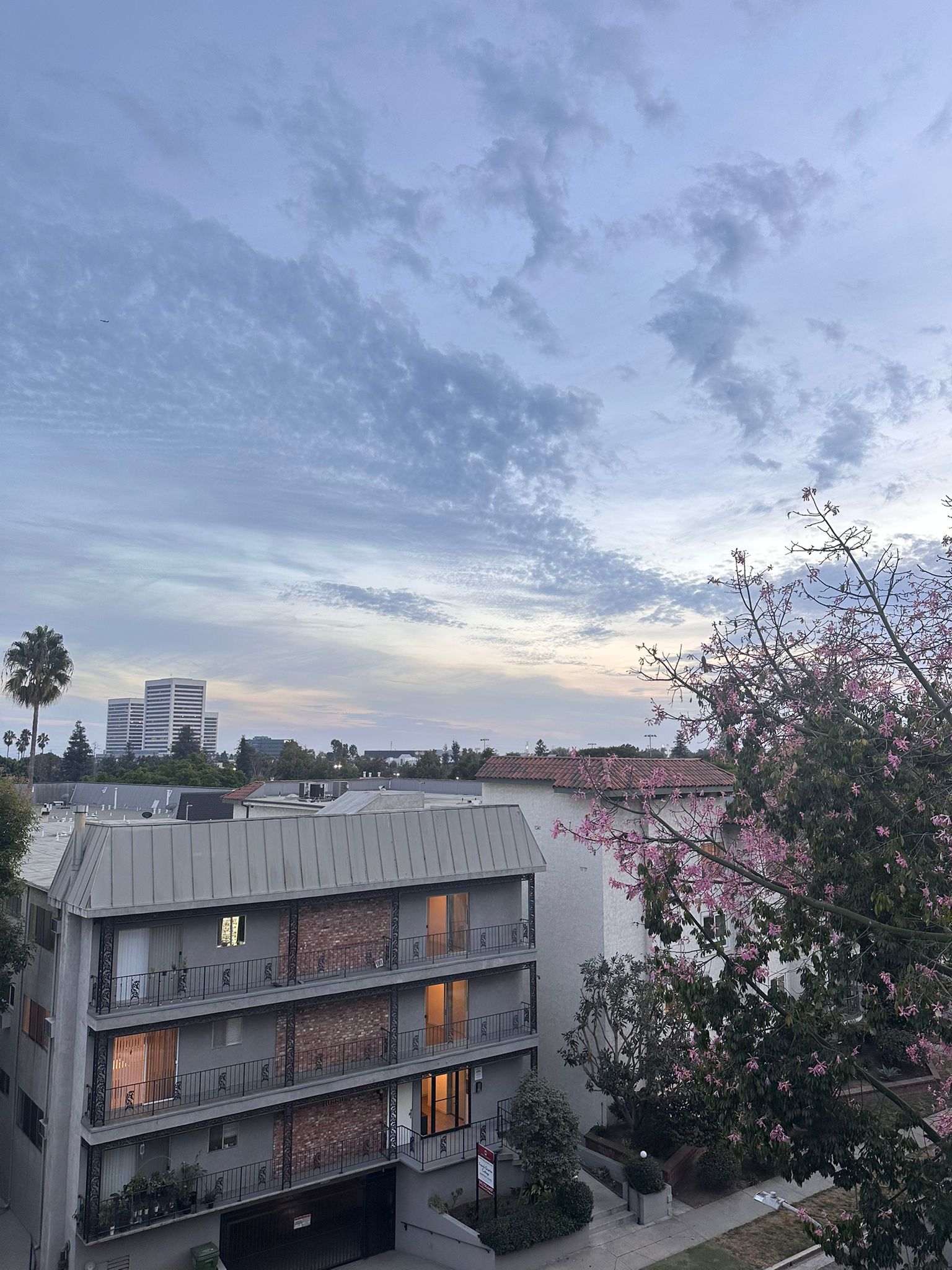
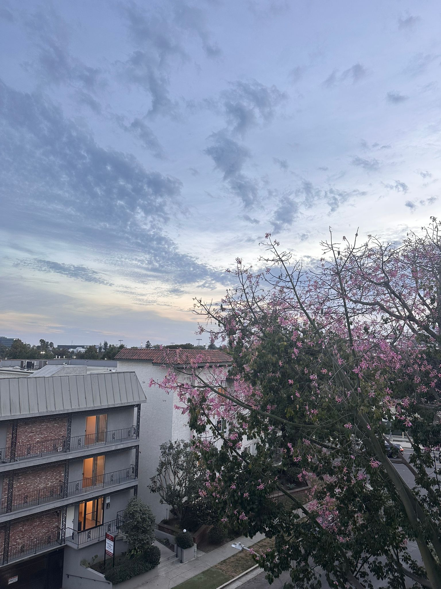
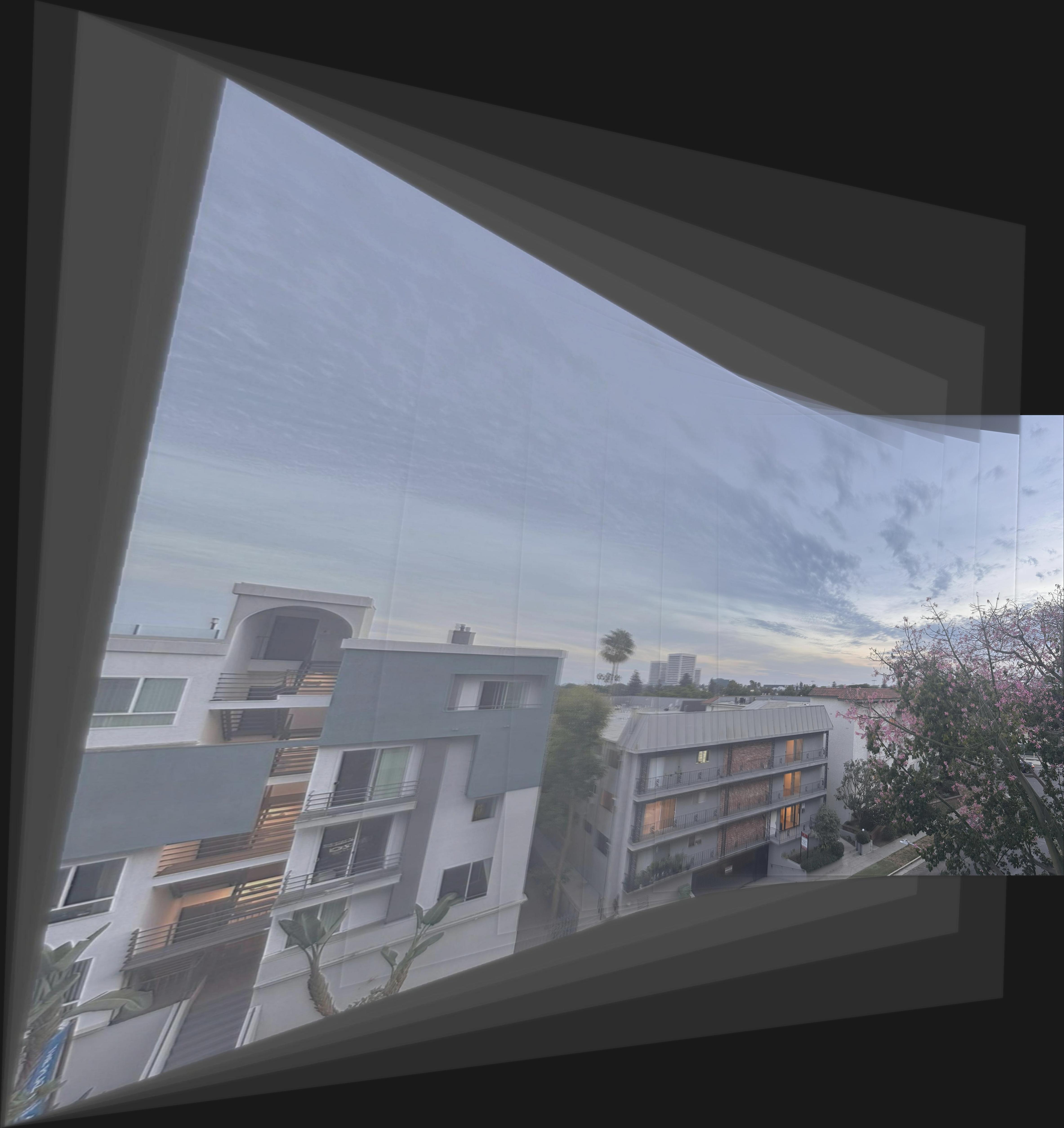
Zoom out with (CMD-) after clicking on the image
5'o clock coffee in front of Wurster - p1
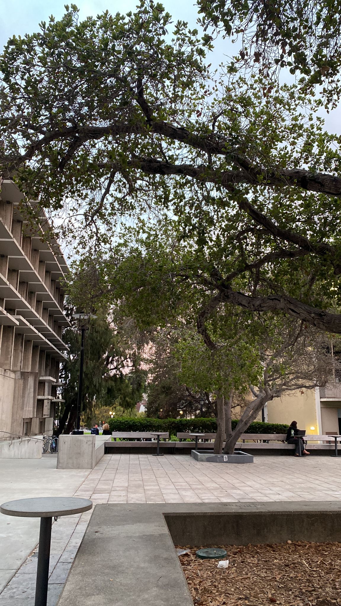
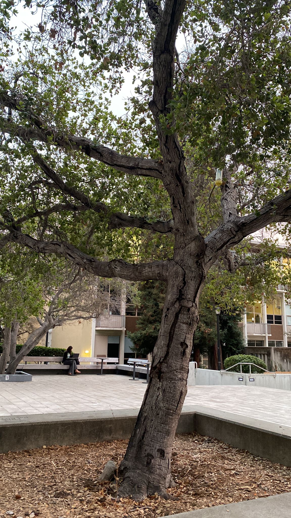
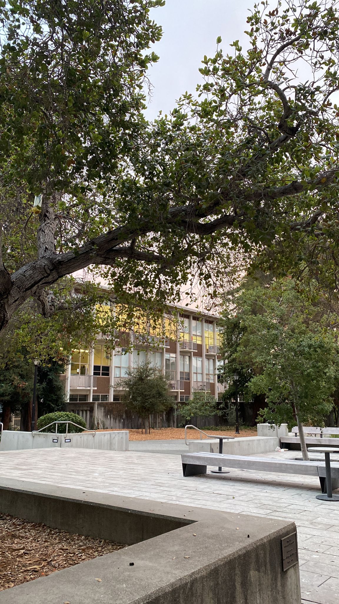
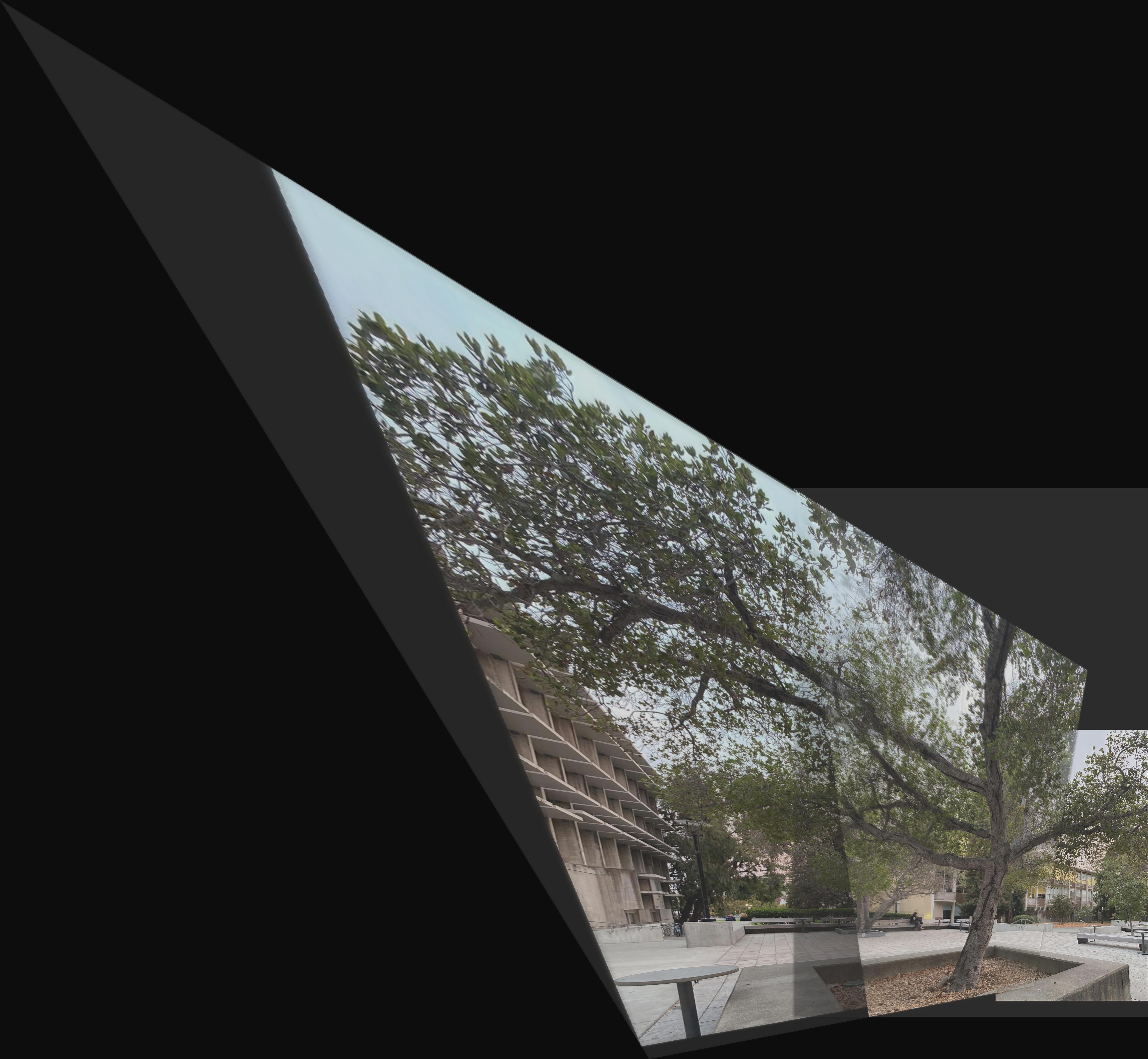
Zoom out with (CMD-) after clicking on the image. Initial pictures were slightly unideal for panoramas
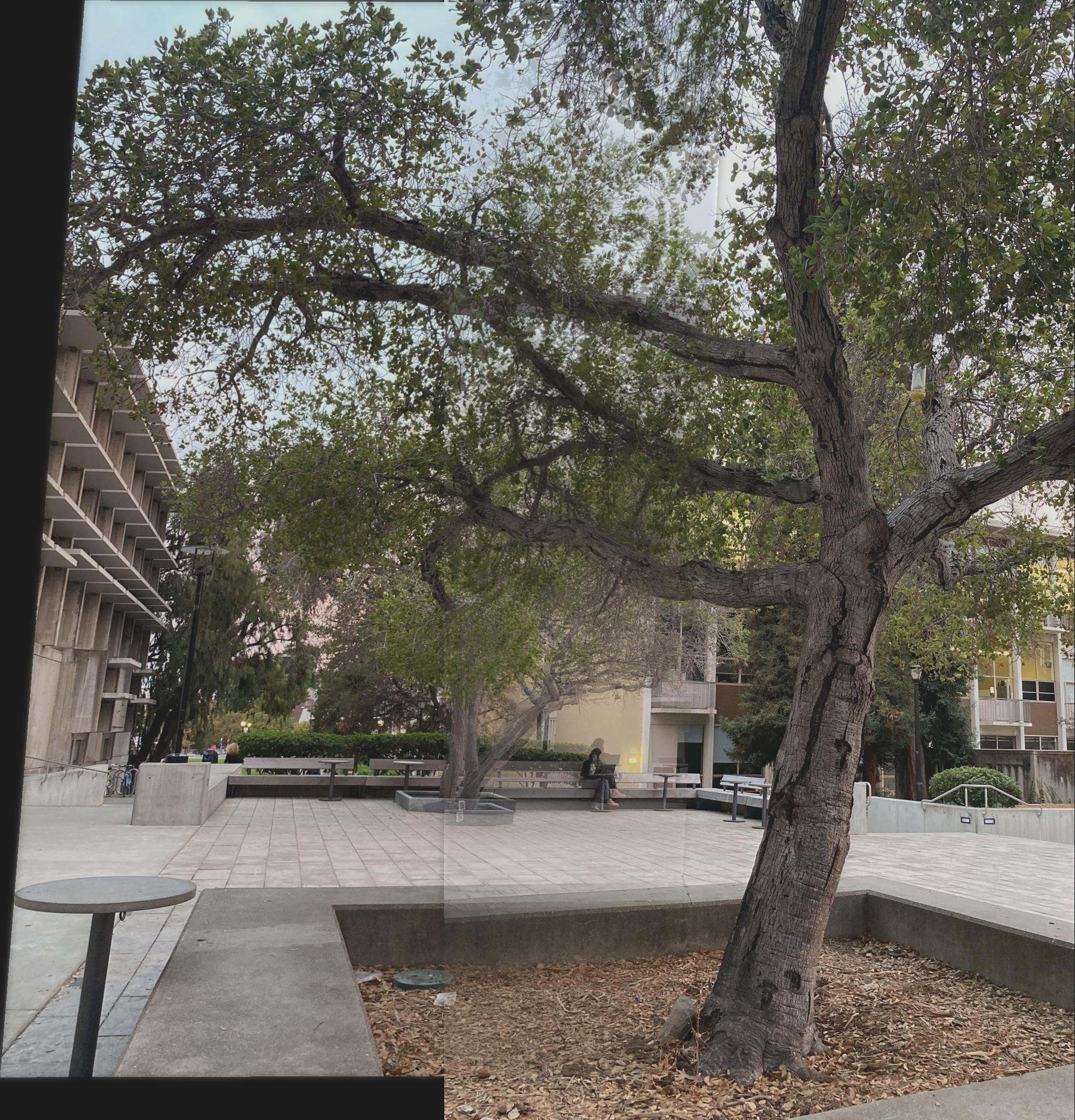
Not the full image, but better results since more appropriate starting images
5'o clock coffee in front of Wurster - p2
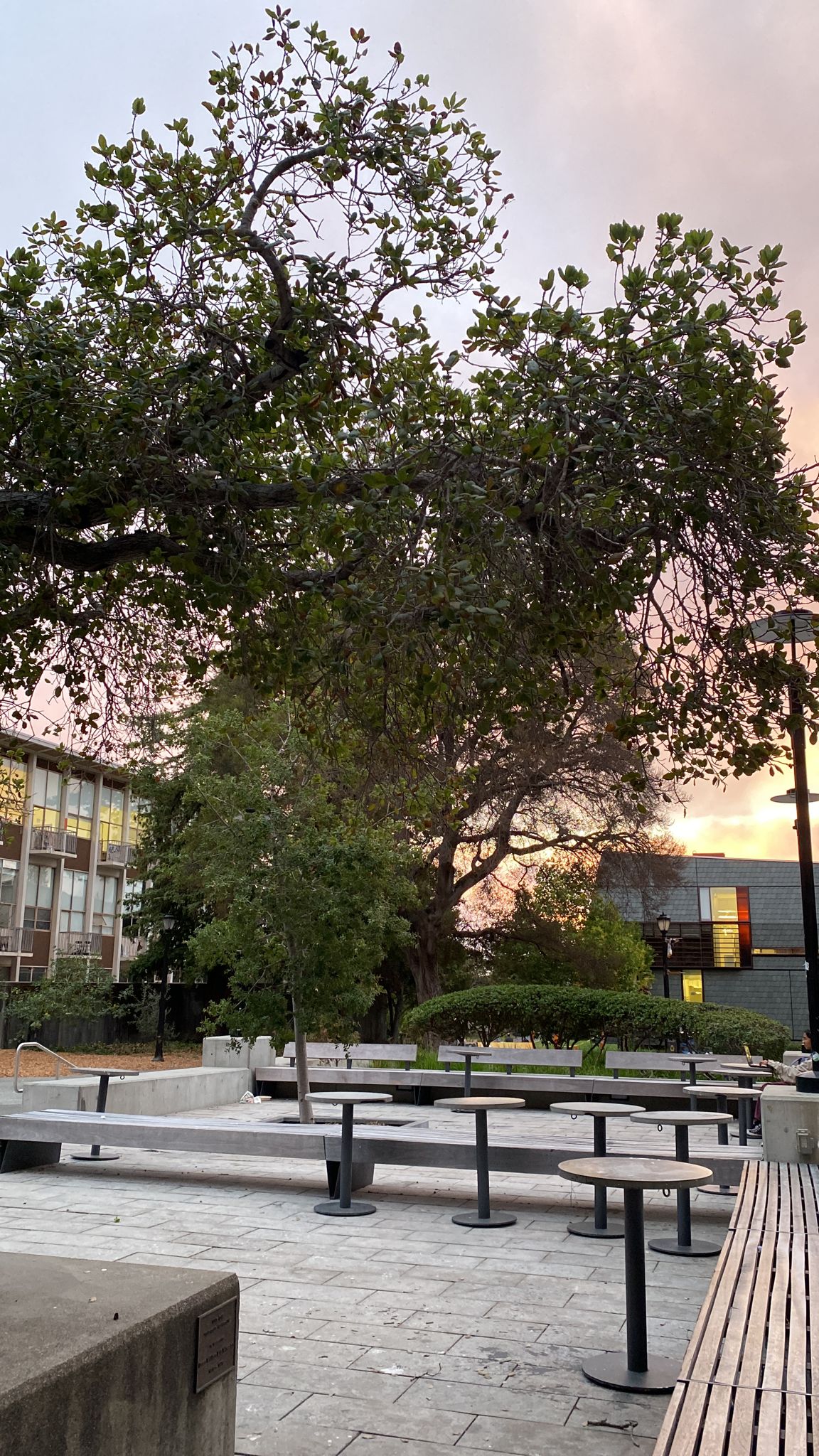
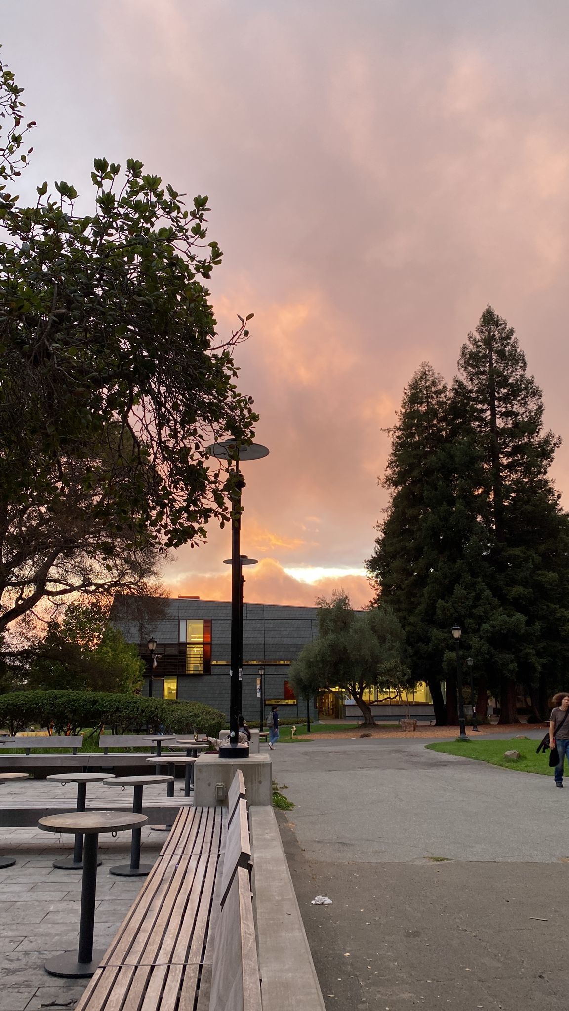
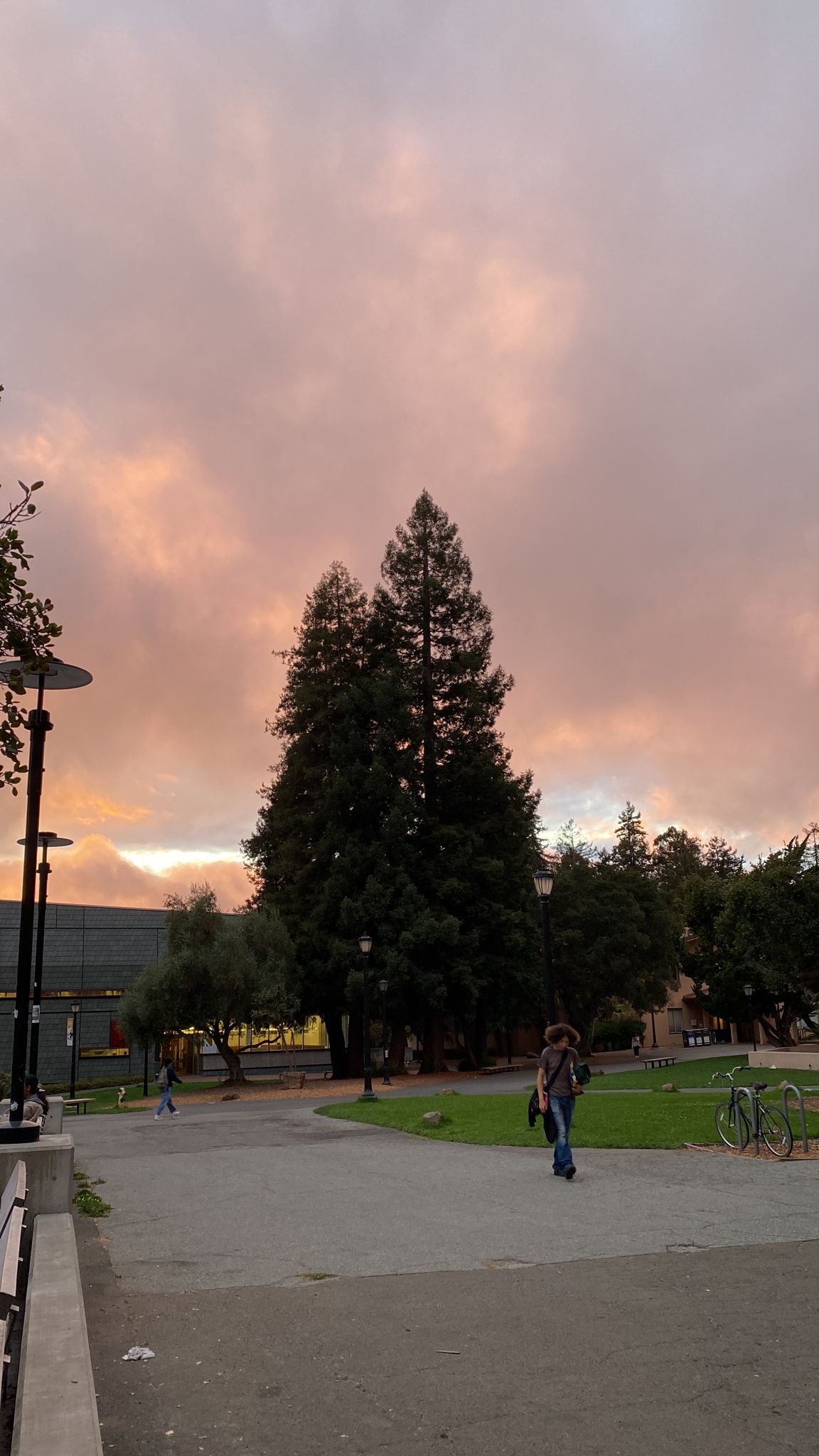
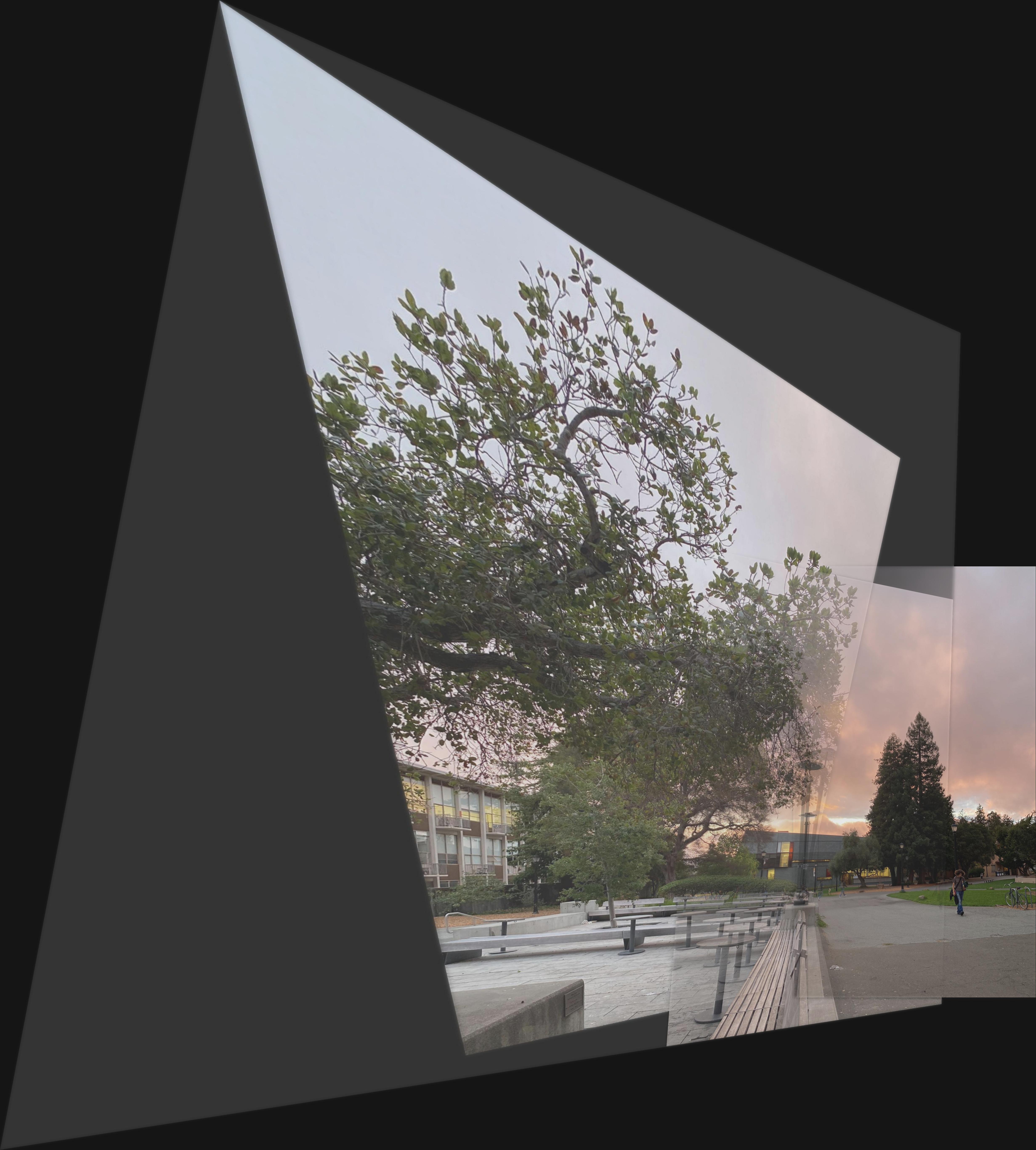
Zoom out with (CMD-) after clicking on the image. Initial pictures were slightly unideal for panoramas
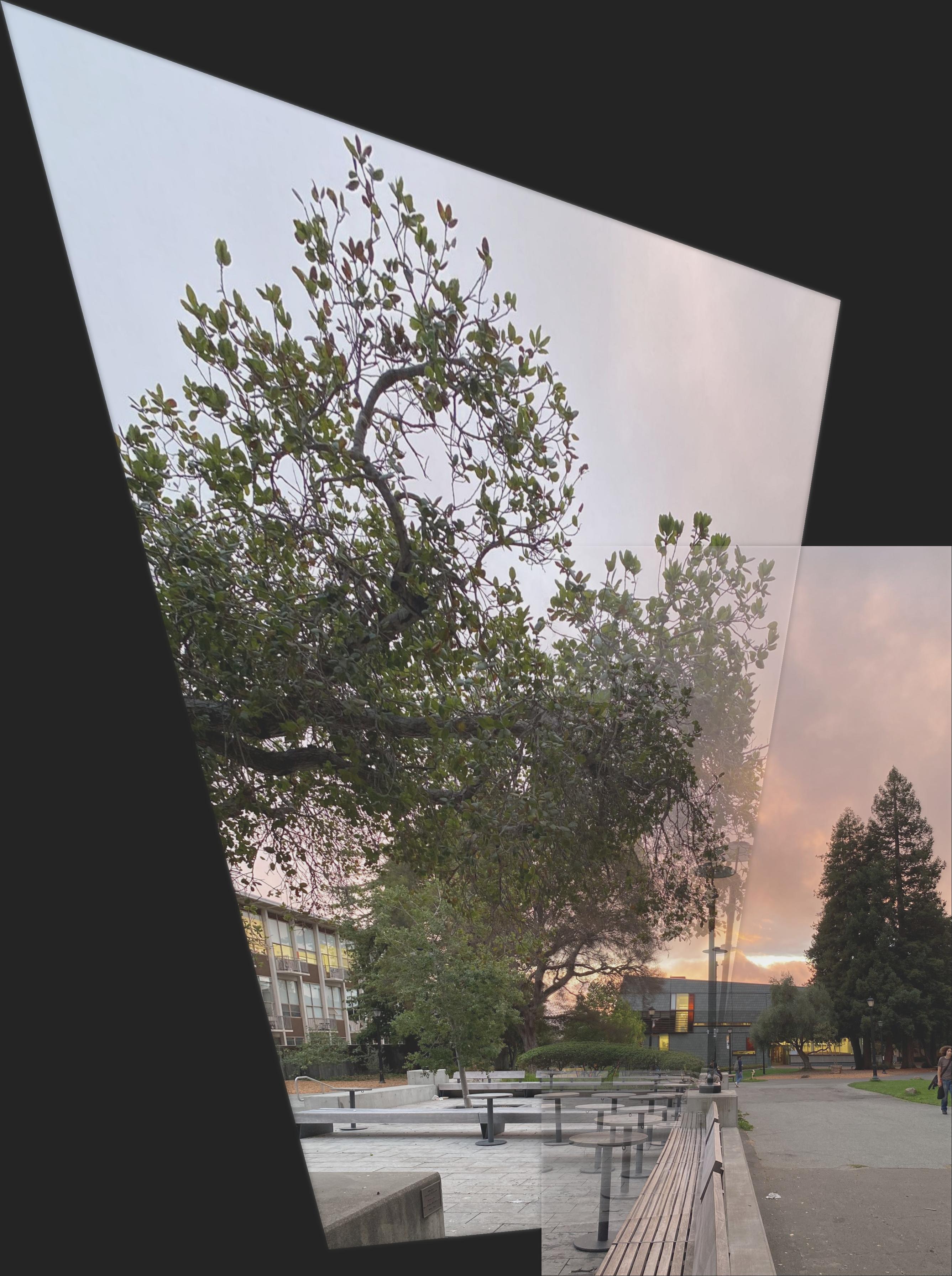
Not the full image, but better results since more appropriate starting images
Office View - (This time automatic)


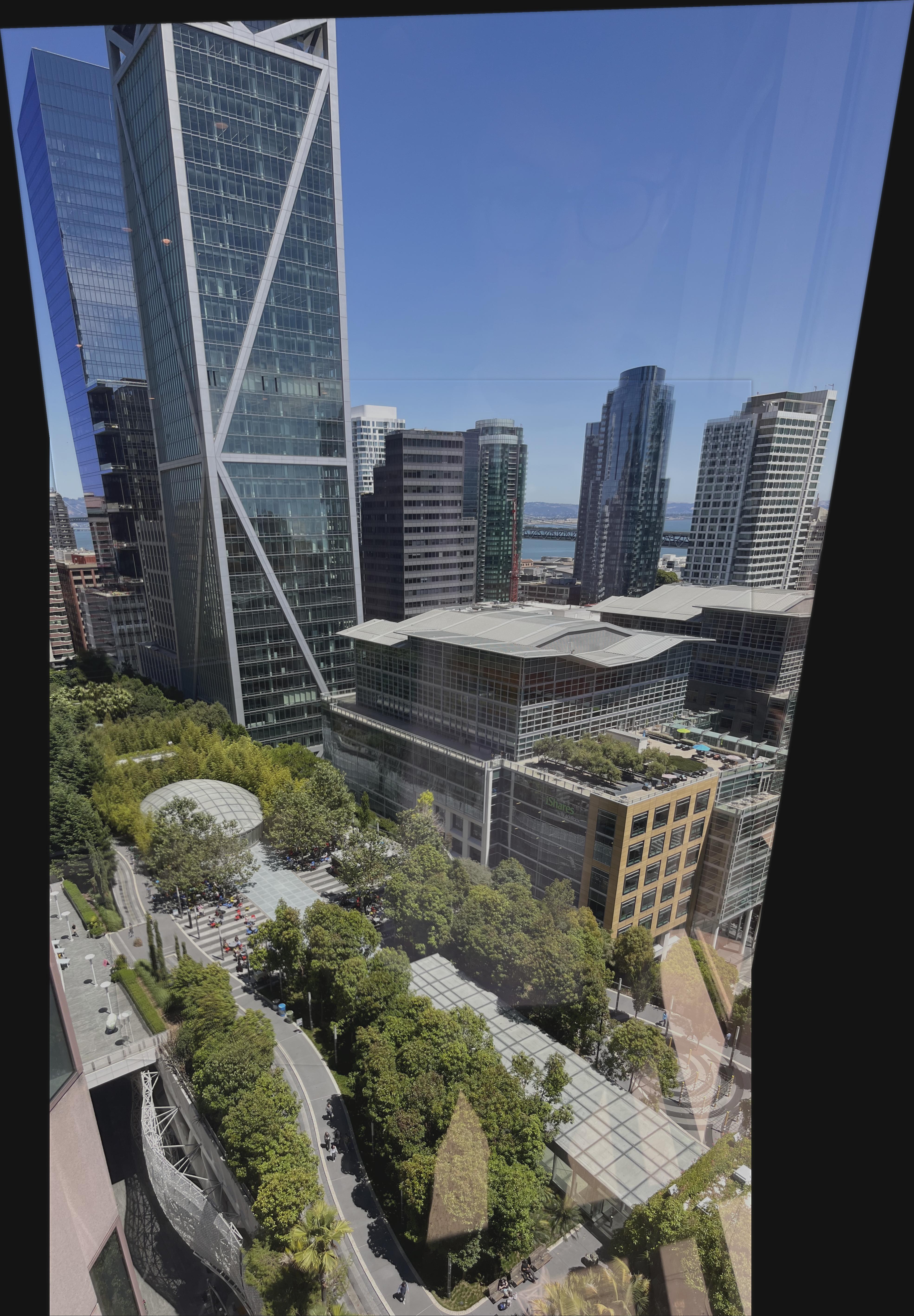
Zoom out with (CMD-) after clicking on the image