CS180 Project 2: Fun With Filters and Frequencies
Deniz Demirtas
In this project, we experience with creation and applications of various filters for different image processing tasks. Come on to a journey of learning with me!
Part 1: Fun with Filters
Part 1.1: Finite Difference Operator
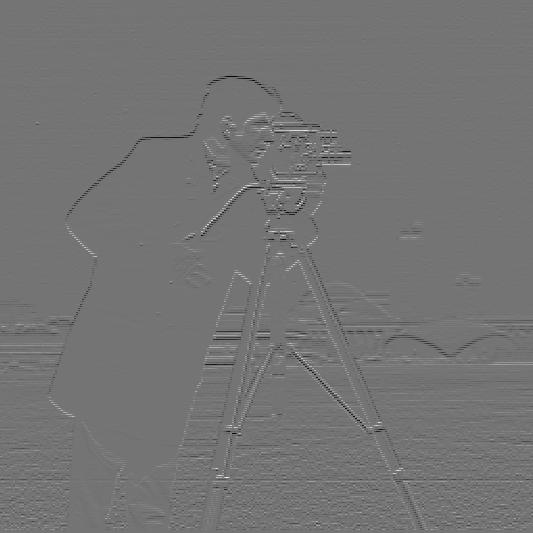
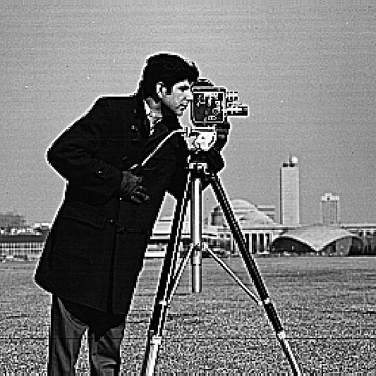
For this section, we are tasked with applying finite difference operators to our image to detect
edges. Specifically, we use D_x = [1, -1] for horizontal edges and
D_y = [1, -1]^T (where ^T denotes the transpose, making it a column
vector) for vertical edges. Intuitively, convolving the image with D_x detects
changes in the horizontal direction, indicating vertical edges, and conversely, convolving with
D_y detects changes in the vertical direction, indicating horizontal edges. This
can be thought of as observing the incremental changes in the image as if moving stepwise in one
direction reveals edges perpendicular to that direction.
Partial Derivatives
Horizontal edges

Vertical Edges
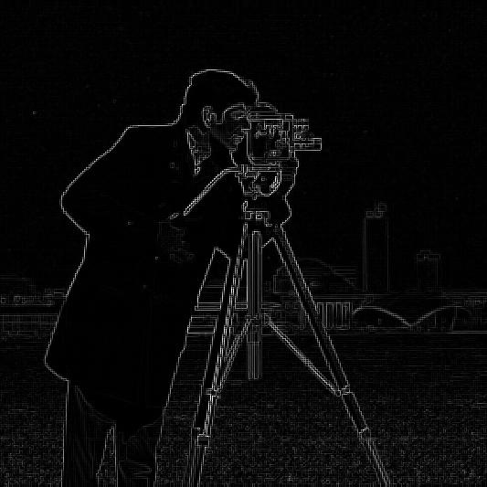
Now, to turn the partial derivatives into an edge image, I have calculated the gradient magnitude
image. The gradient magnitude is computed by taking the square root of the sum of the squares of
the partial derivatives in both the x and y directions. This value represents the rate of change
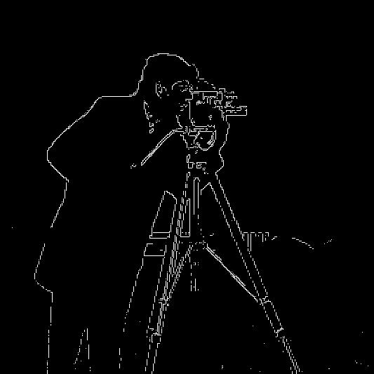
at each point in the image, highlighting the edges. After computing the gradient magnitude, I
binarized it with an empirically tested threshold 0.355 to reduce the noise in the
edge image.
Gradient Magnitude Image
Binary Edge Image
Part 1.2: Derivative of Gaussian (Dog) Filter
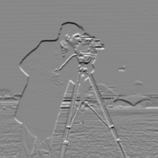
From the lecture, we have learned that convolving the original image with an appropriate Gaussian
filter
would stabilize the gradient computations by smoothing out the original image and enhances the
true edges. Therefore,
I have created a 2D Gaussian filter with the following parameters after following the in-class
advice with some
empirical testing kernel size = 11, sigma = 1.8
Horizontal edges of image smoothened with Gaussian filter

Vertical edges of image smoothened with Gaussian filter
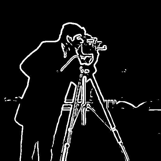
To calculate the gradient binary image, after empirically testing threshold values, I have
settled at 0.31

Gradient magnitude of image smoothened with Gaussian filter
Binary gradient magnitude of image smoothened with Gaussian filter
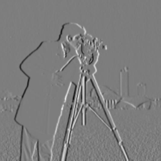
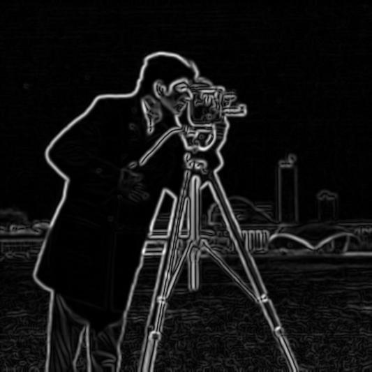
Now, we understand that identical results can be achieved by convolving the Gaussian filter with
D_x and D_y respectively instead of convolving the image with the
Gaussian filter,
and then convolving with finite difference operators onec again, thanks to the associativity of
convolution.
By visually comparing the results below with the above version, we can confirm this.

Horizontal Edges after DoG convolution
Vertical Edges after DoG convolution
Gradient magnitude image after DoG convolution

Binary gradient image after DoG convolution
Differences Between Part 1.1 and Part 1.2 Outputs
Starting from the visual differences observed in the gradient magnitude image, the edges appear more continuous than the discrete edges seen with the initial edge detection method. Besides the more continuous appearance, the edges in the image are thicker, and patterns resembling noisy artifacts are more pronounced. The main takeaway is that the image appears smoother compared to how it looked more pixelated previously. As for the binary edge image, the results show smooth, continuous edges that focus strictly on the image content, significantly reducing noise. Additionally, the background edges are captured more clearly.
DoG Filters Used Visualized

DoG_x

DoG_y
Part 2
Part 2.1: Image "Sharpening"
An unsharp mask filter can be implemented in a single convolution operation by designing a specialized convolution kernel that combines both Gaussian blurring and edge enhancement. This kernel features a central positive coefficient, which is significantly higher than the sum of the surrounding negative coefficients. When applied to an image, this kernel simultaneously blurs and sharpens by subtracting a fraction of the blurred image from the original. The central positive weight enhances the contrast of central pixel values relative to their neighbors, accentuating edges. This approach allows for a streamlined, efficient process that achieves edge sharpening and detail enhancement in one convolution step.
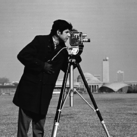
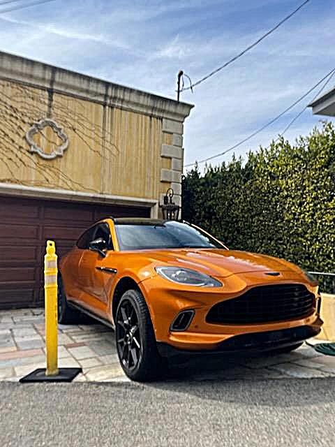
When deciding which images to experiment with, I recalled a time as a car enthusiast when I spotted a car but was unsuccessful in capturing clear images because the car I was in was moving. This presented a perfect opportunity to apply my academic knowledge to enhance my daily life. Here are the results of my images adjusted with different alpha values.
Original Image

alpha = 2
alpha = 4

alpha = 6
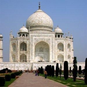
Original Image
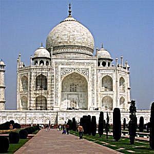
alpha = 2
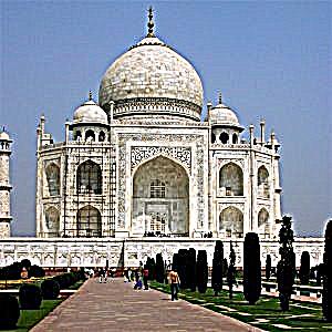
alpha = 4
alpha = 6

Original Image

alpha = 1
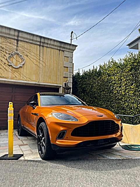
alpha = 2
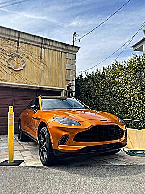
alpha = 4

Original Image
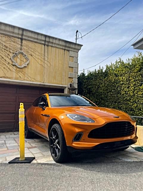
alpha = 1
alpha = 2

alpha = 4
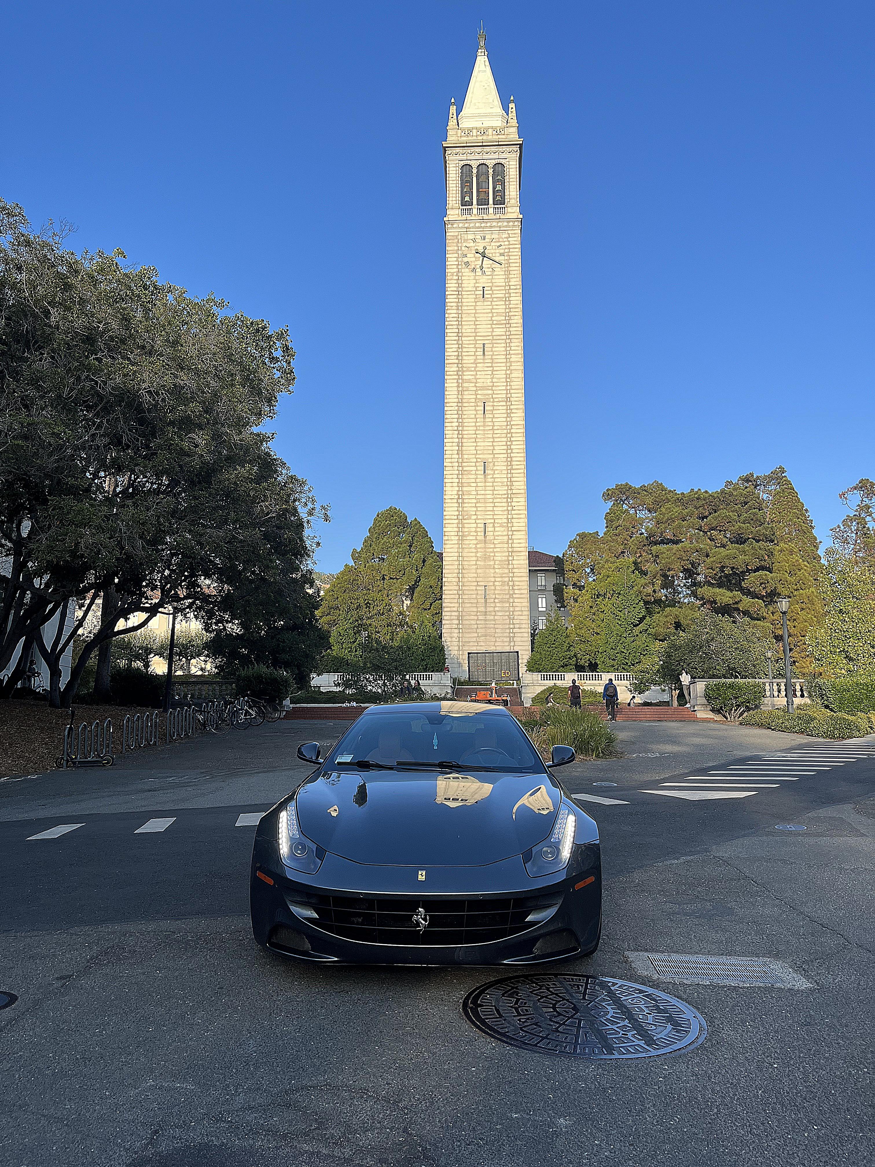
The results at low alpha are great. Here is an experiment with an image that's already sharp enough.

Original Image

alpha = 1

alpha = 2
alpha = 4
The results of the unsharp mask filter show that it makes the edges more pronounced. Additionally, the level of sharpness can make the image appear pixelated to the eye, due to the further emphasis and smaller size of perpendicular edges. However, there isn't much sharpening being achieved as the alpha increases compared to other images.
Part 2.2: Hybrid Images
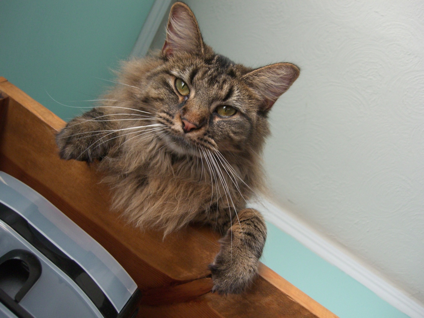
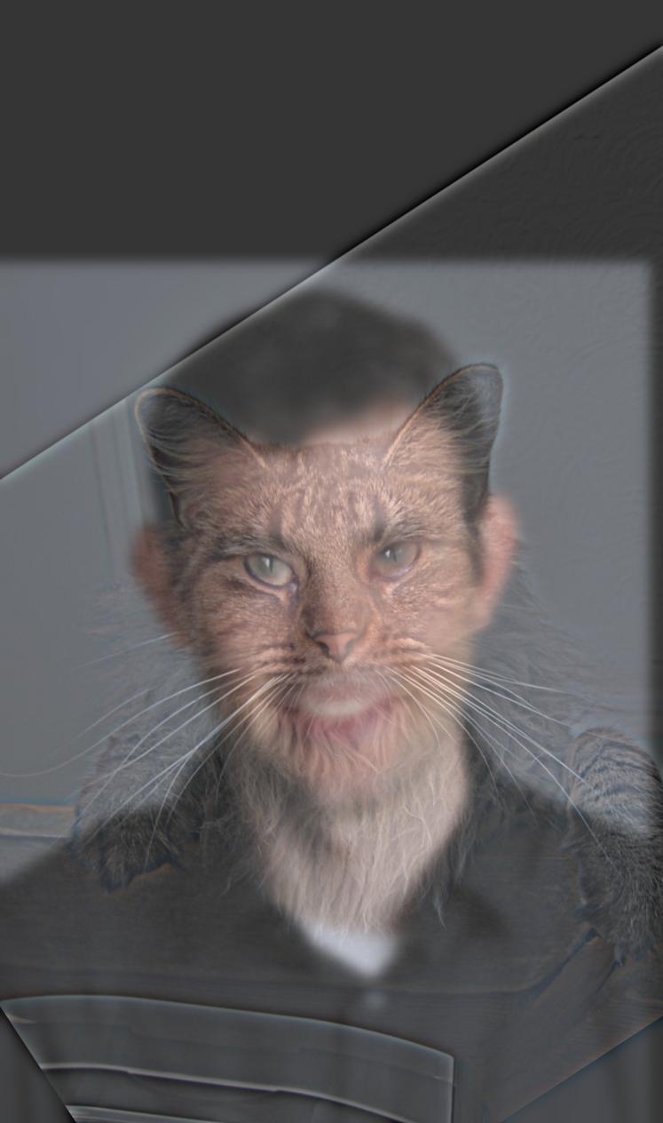
Hybrid images are images where what you see changes depending on the distance you view them from. This happens because two images are encoded into one: one image's high frequencies and the other image's low frequencies. Our eyes are better at picking up high frequencies when viewing up close, but as we move farther away, we begin to perceive the image with lower frequencies. Therefore, up close, we see the image with higher frequencies, and from a distance, the lower frequency image becomes more prominent. Here are a few examples.
Derek and Nutmeg

Original Derek
Original Nutmeg
Hybrid Image
Frenemies - Meme that would get me in a Turkish Jail (Favourite)
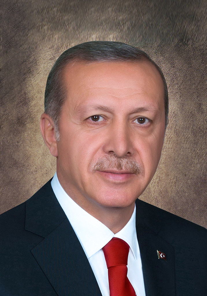
Original Erdogan (president)
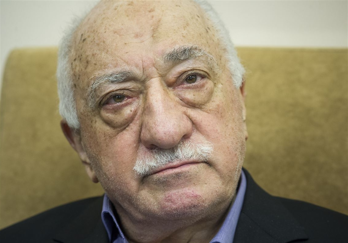
Original Gulen (leader of the failed coup)
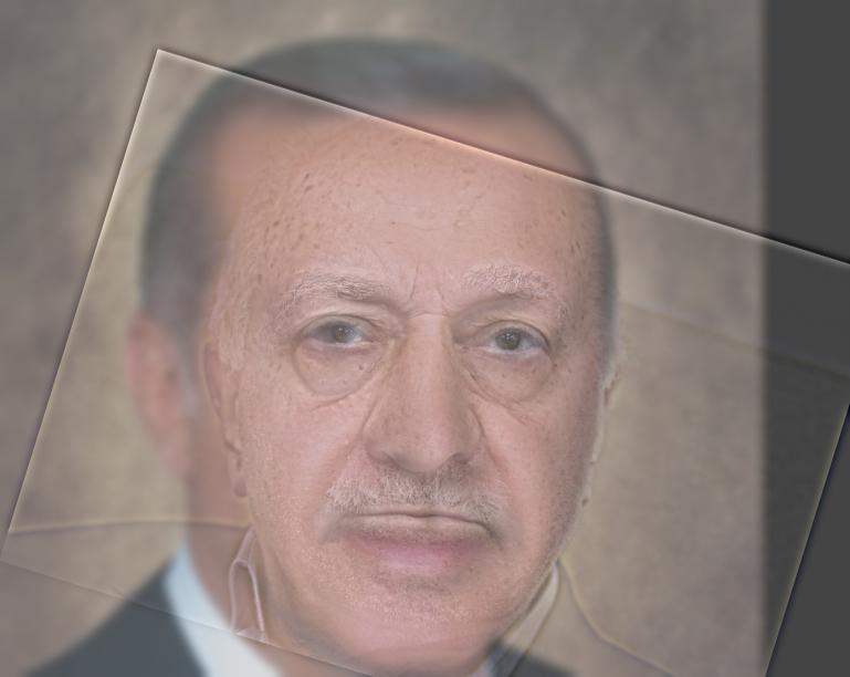
Hybrid Image (frenemies)
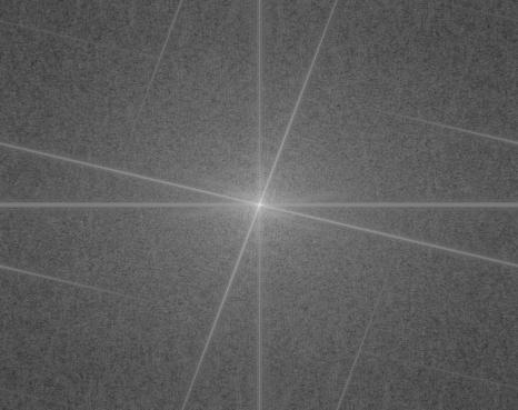
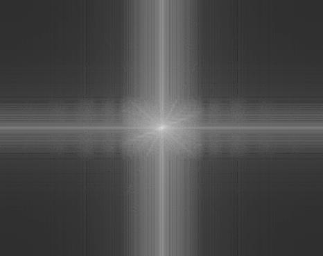
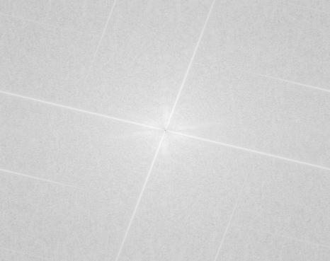
Frequency Analysis
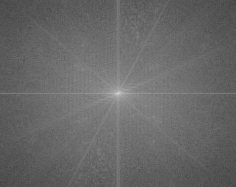
Original Erdogan FFT
Original Gulen FFT
Erdogan Low Pass Filtered FFT
Gulen High Pass Filtered FFT
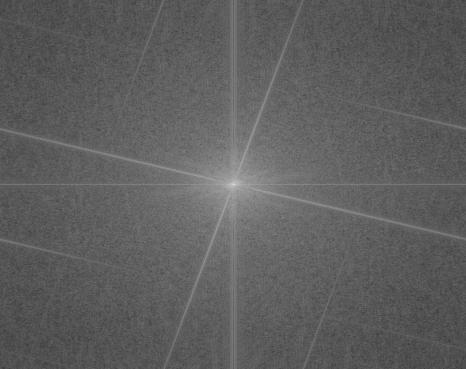
Hybrid Image FFT
Make art not war - (failure, arguably ?)
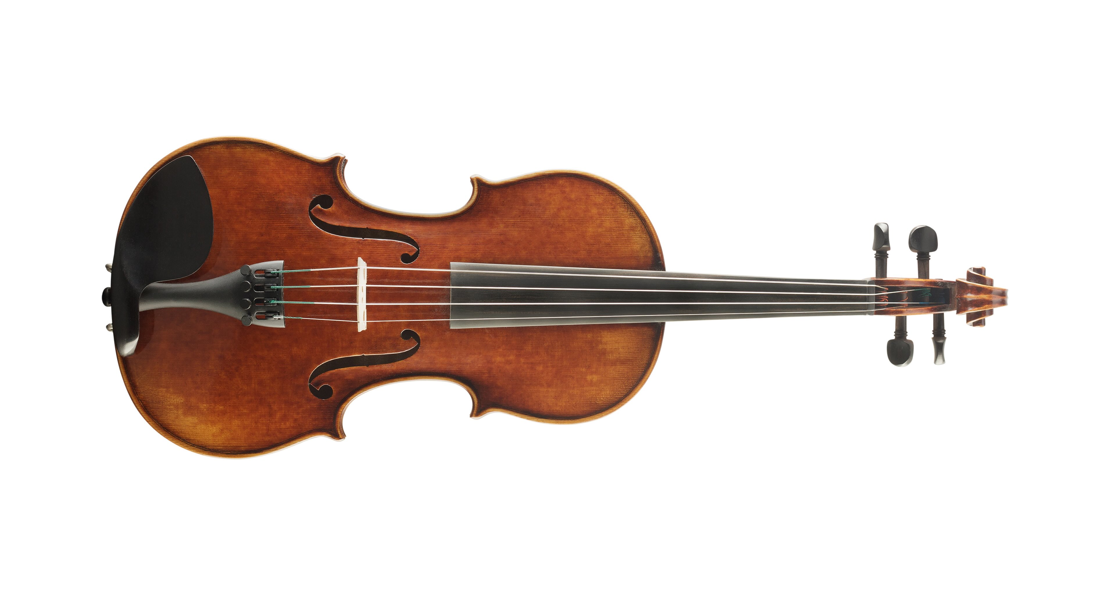
Original Violin
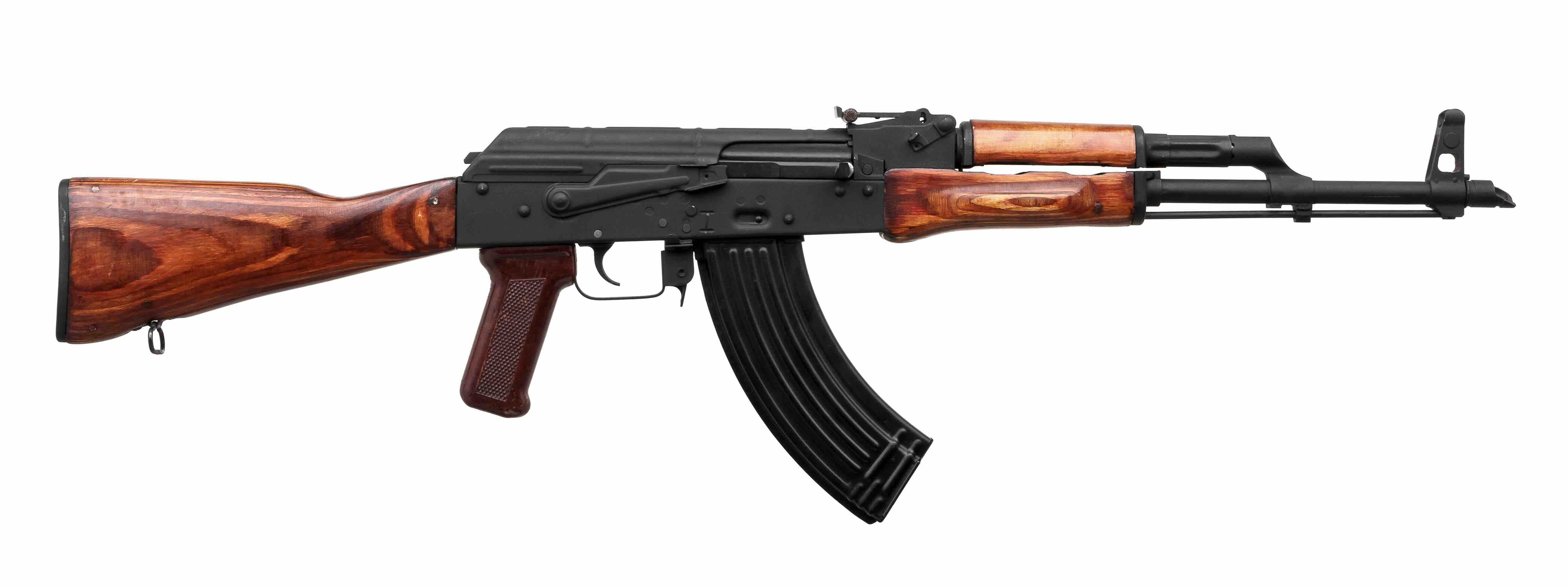
Original Gun
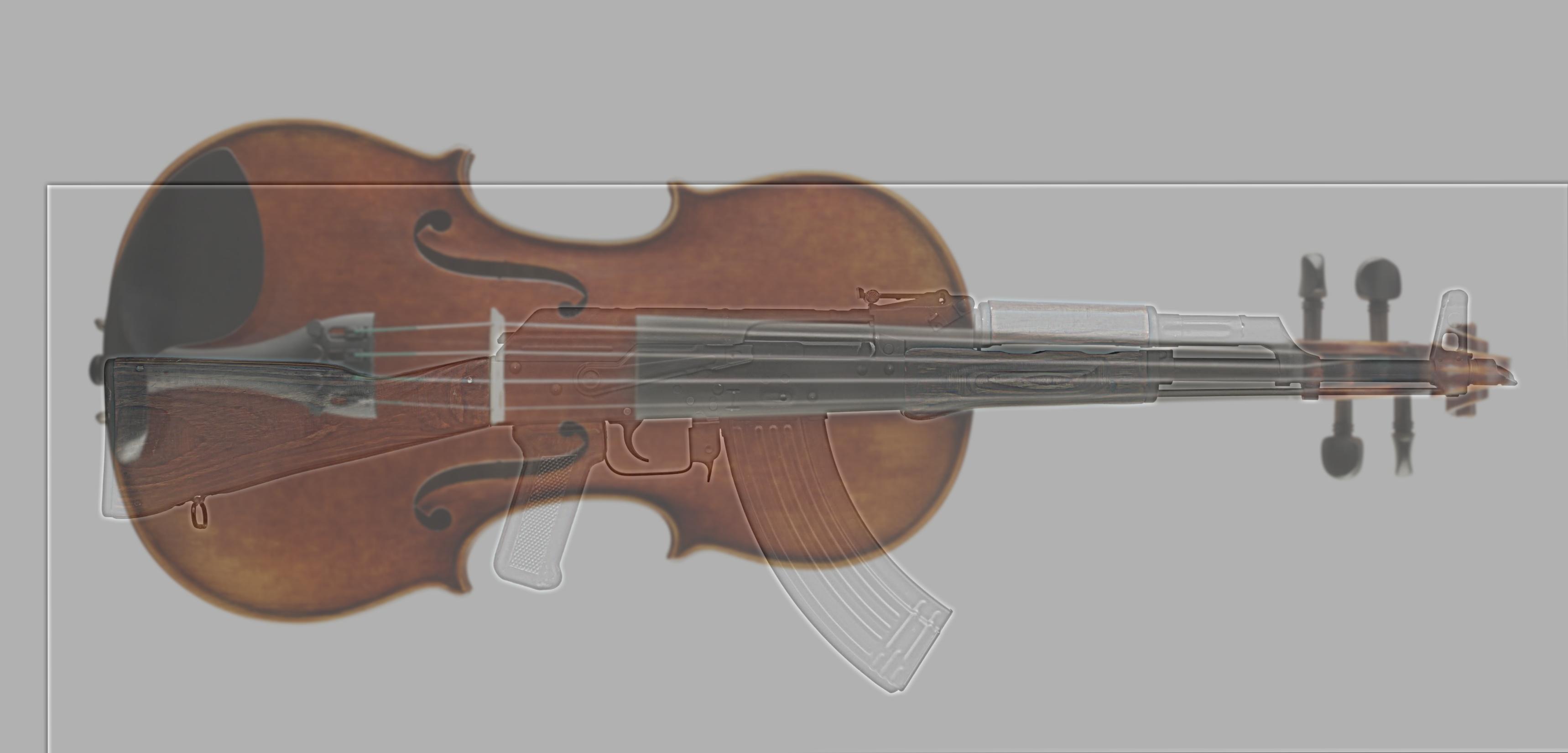
Hybrid
Part 2.2 - Bells & Whistles
For the bells and whistles part, I wanted to give the "Make art not war" image a chance since it's results can definitely use some improvements. In my opinion, there is no clear winner, it's up to the viewers' taste.
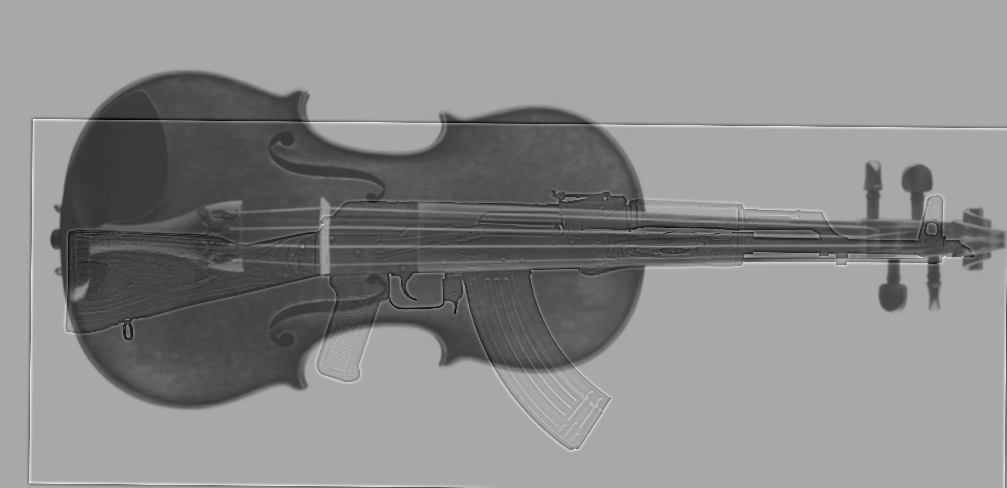
Low Frequency Image grayscale, high frequency image colored
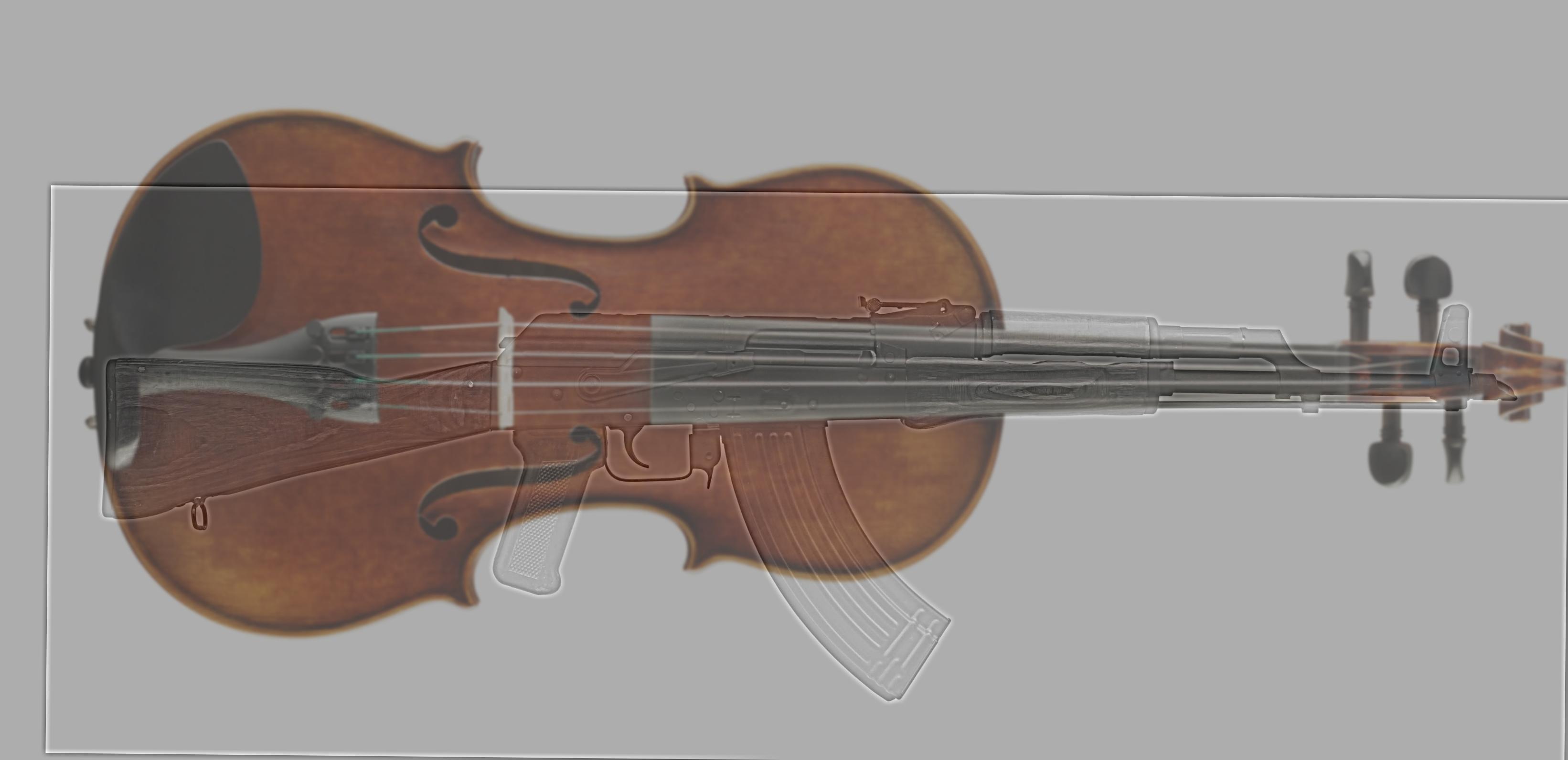
High Frequency Image grayscale, Low frequency image colored
Part 2.3: Multi Resolution Image Blending
Image blending is a powerful technique used to seamlessly merge two images, creating a smooth and natural transition between them. This is achieved by generating a transition region, or mask, that gradually blends one image into the other. The blending process operates across multiple levels of detail, or frequency layers, of the images. By utilizing Laplacian and Gaussian pyramids, the technique ensures that both coarse and fine details are blended harmoniously, resulting in a visually consistent output. The Gaussian pyramid is used to create progressively blurred versions of the images, while the Laplacian pyramid captures the high-frequency details, allowing for smooth transitions even at the smallest scales.
Original Images
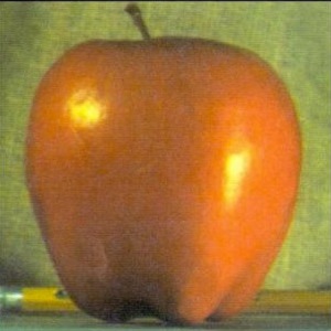
Apple
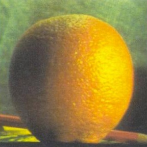
Apple
The process begins by constructing the Gaussian pyramids for both images. At each level of the pyramid, the images undergo Gaussian blurring followed by subsampling, progressively reducing the image resolution. This technique effectively isolates different frequency bands at each level, allowing us to access a broad range of image details. The lower levels capture the high-frequency, fine details, while the upper levels focus on the low-frequency, large-scale structures, providing a comprehensive representation of the image across multiple spatial frequencies.
Gaussian Pyramids


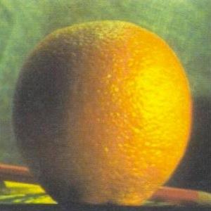


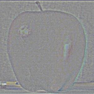
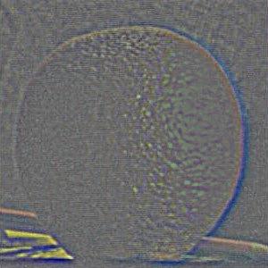
Next, we compute the Laplacian pyramids for both images. This is done by subtracting the current level of the Gaussian pyramid from the upsampled version of the next coarser level. This operation isolates the higher-frequency details at each step, capturing the fine textures and edges that distinguish different levels of detail within the image. By repeating this process across the pyramid, we can systematically extract the high-frequency components that are critical for blending sharp features and preserving image clarity during the merging process.
Laplacian Pyramids




Afterward, we create a Laplacian pyramid by blending each level of the respective image
Laplacian pyramids with the corresponding level of the Gaussian mask pyramid. This is done using
the formula mask_level * image1_level + (1 - mask_level) * image2_level. By
applying this blending process at every level, we effectively merge the frequency details from
both images. This approach ensures that the transition between the two images is smooth across
all frequency bands, significantly enhancing the quality and coherence of the final blended
result.
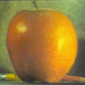
Recreation of Figure 3.42
Level 0
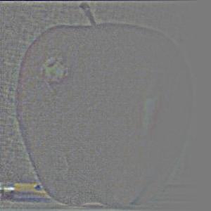
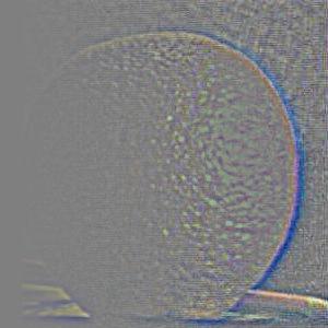
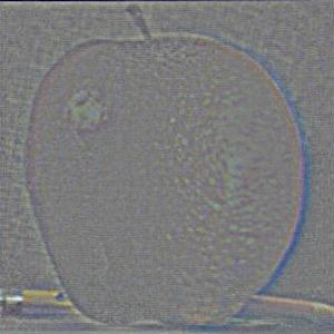
Level 2


Level 4


Final Result
Part 2.4: Multi Resolution Image Blending Results
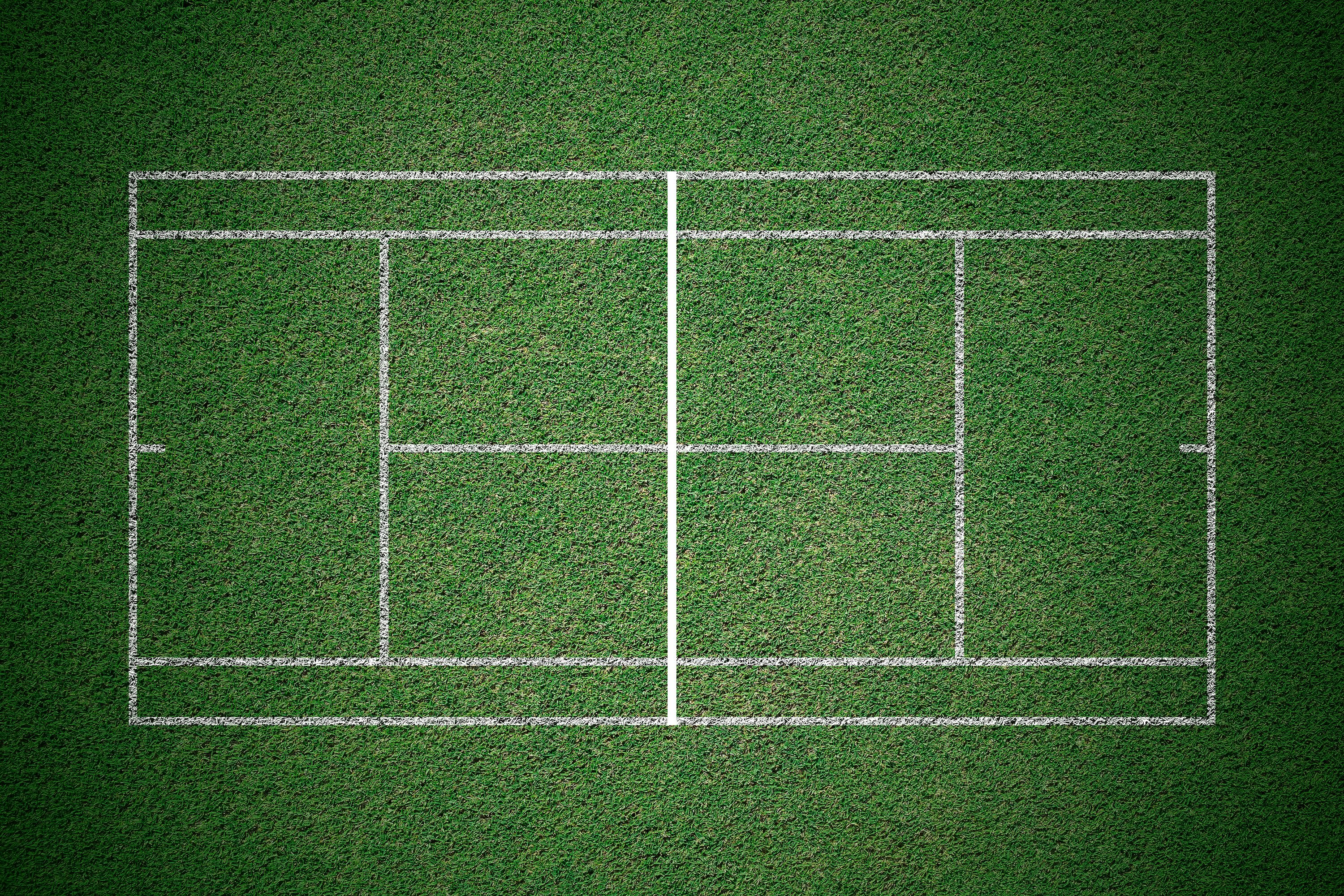
A tribute to the Battle of Surfaces - Federer vs Nadal
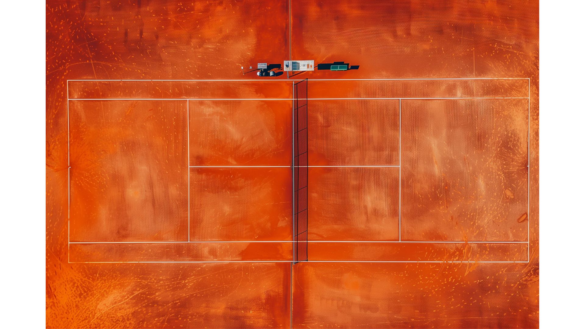
Clay - Nadal
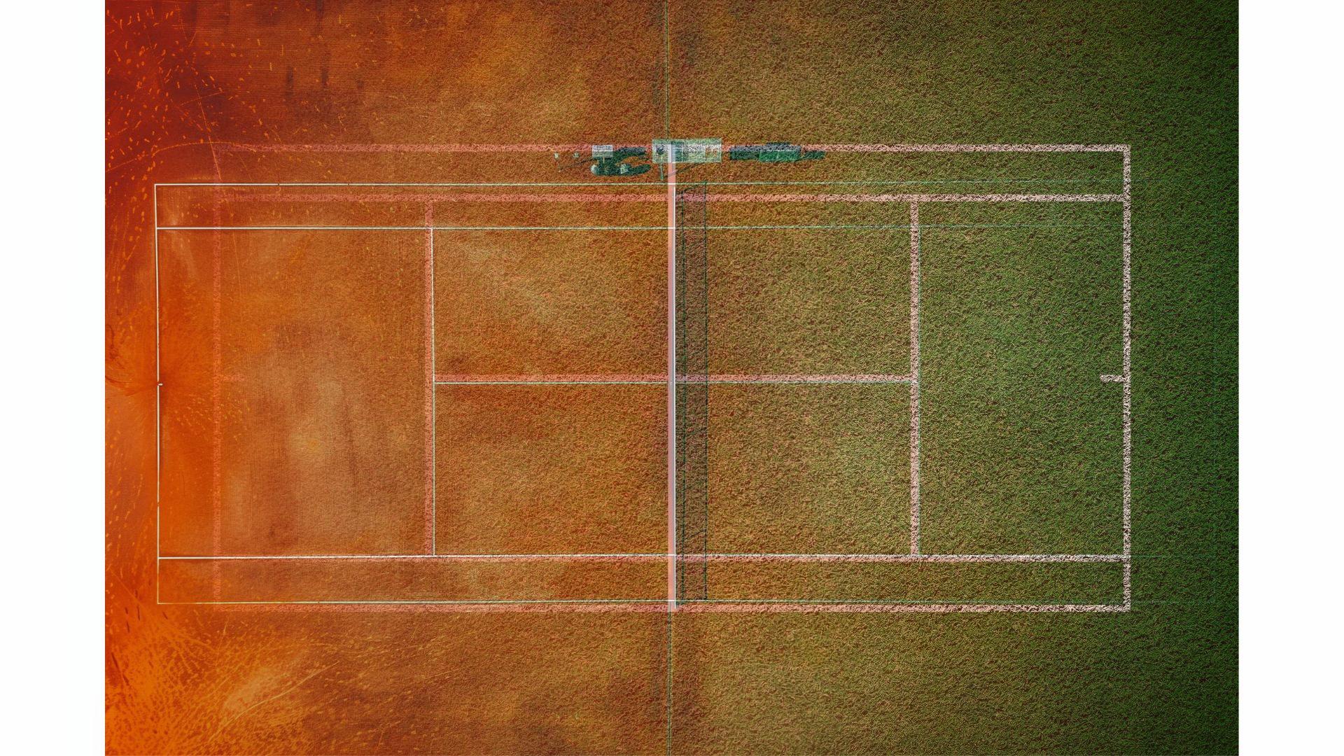
Palma Arena - 2 May 2007
Eggmoji
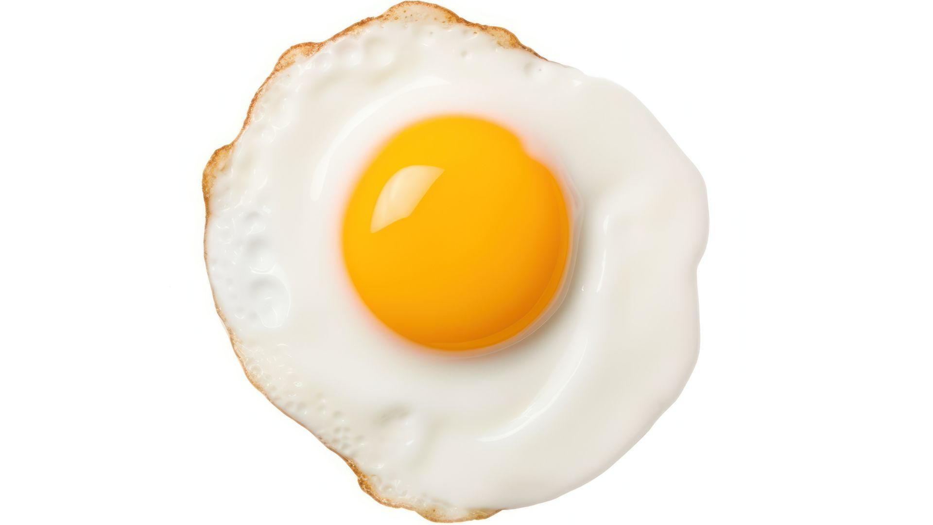

Emoji
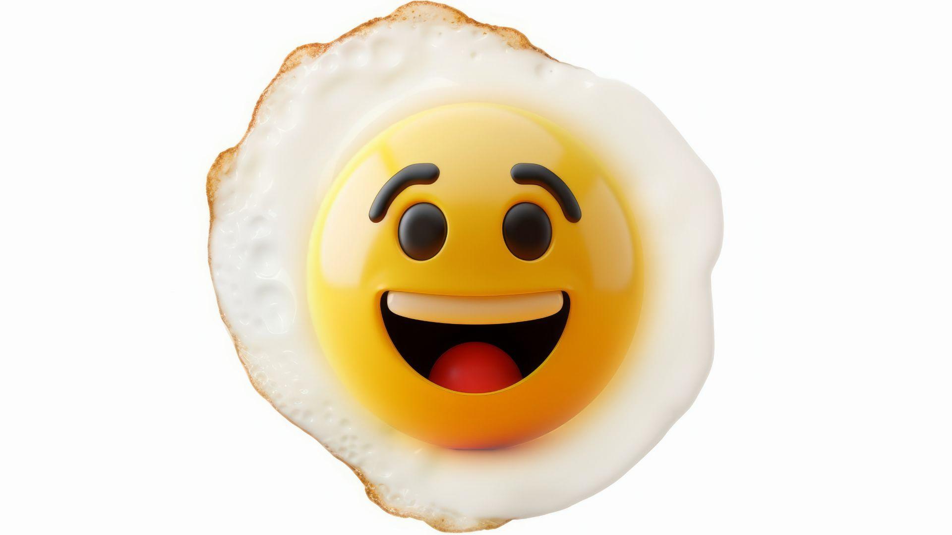
Eggmoji
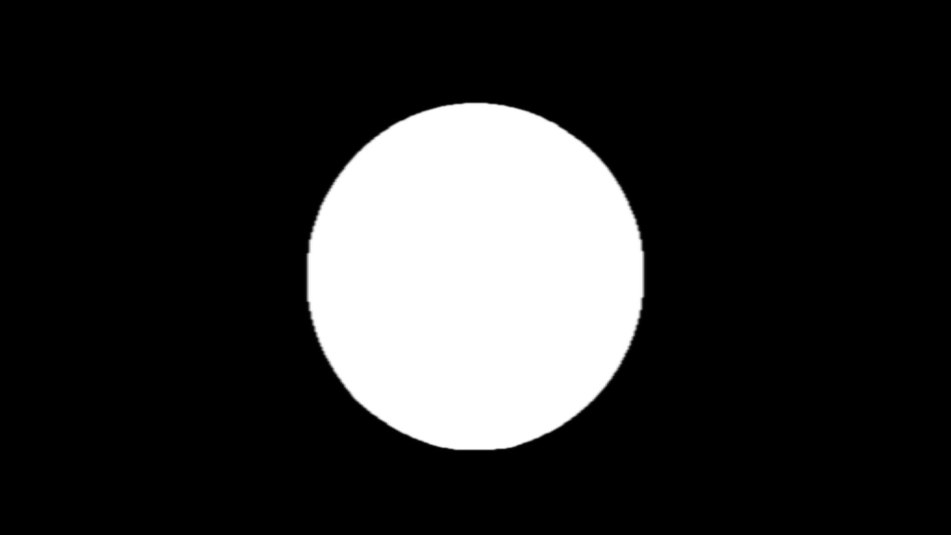
Emoji Mask
My most important takeaway from the project is learning how much the collective frequencies of the image constructs our visual experience. Since we are not able to experience the effects of frequencies, this makes me wonder the signal processing our minds do when blending and creating an image from the incoming frequencies. What type of algorithms does it use?