CS180 Project 1

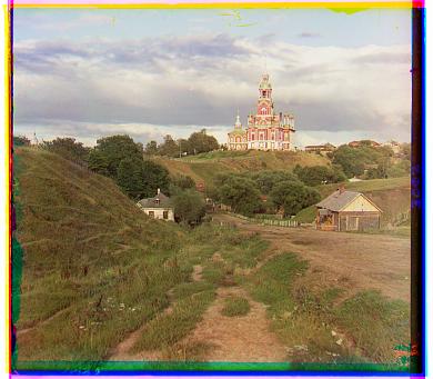
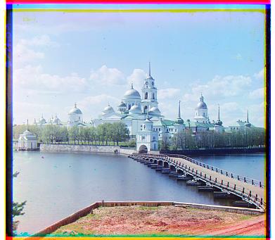
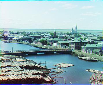
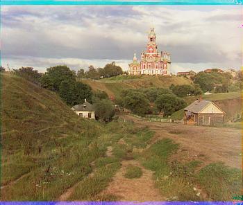
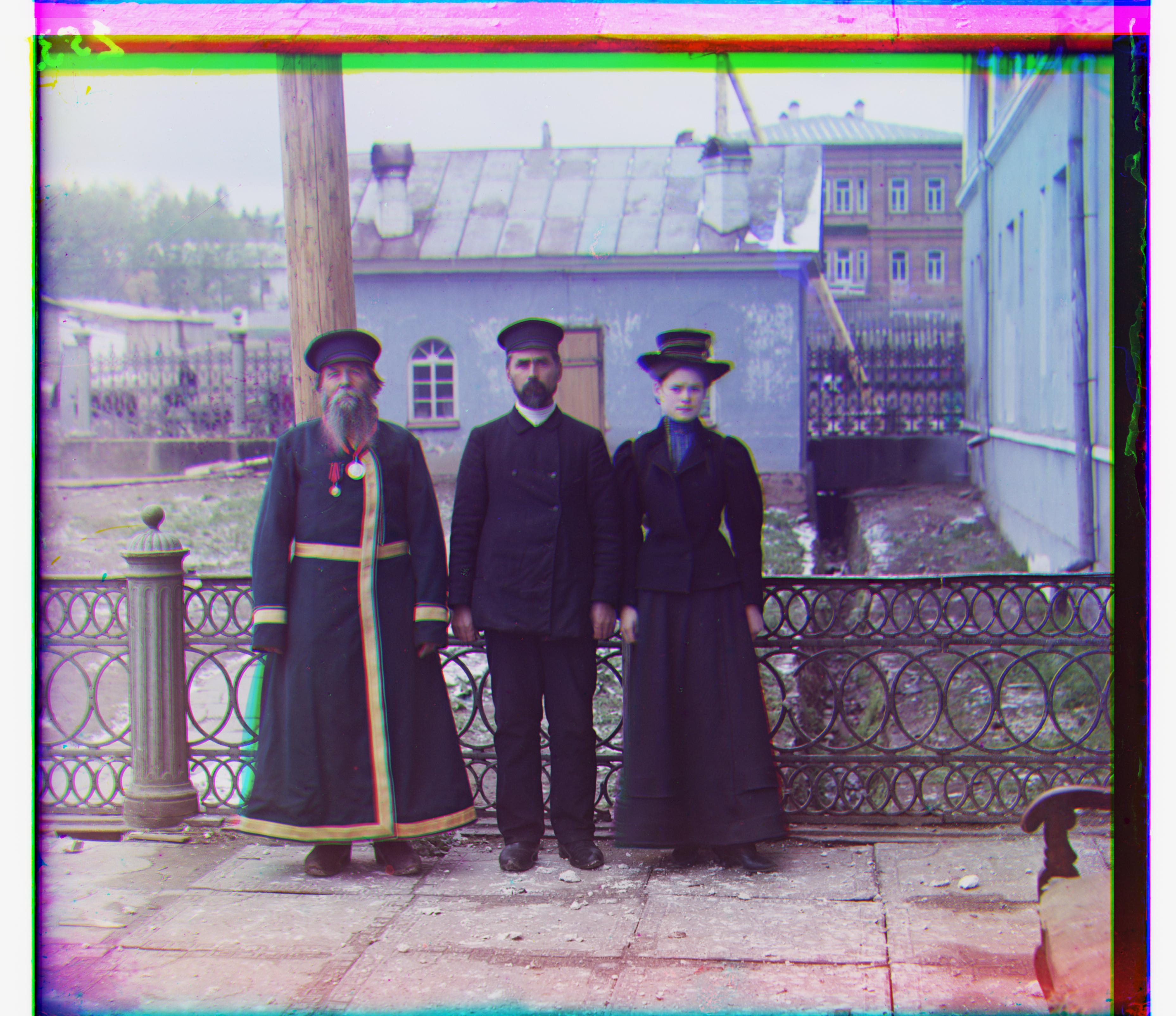
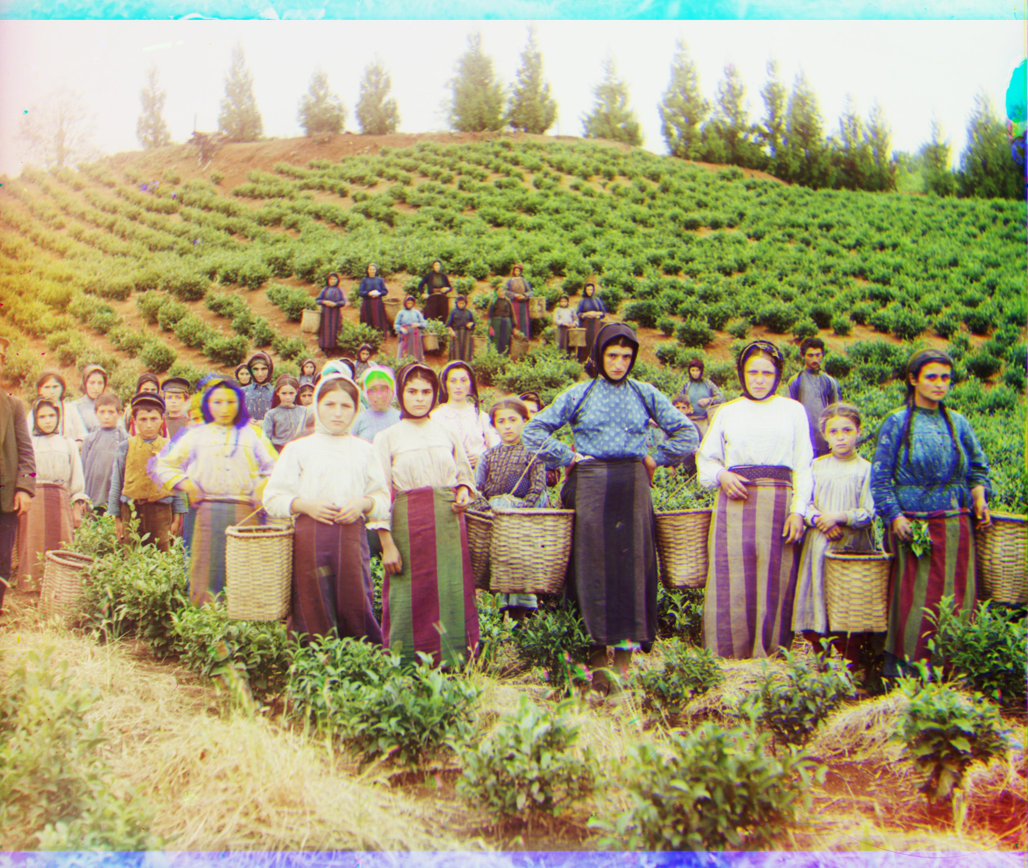
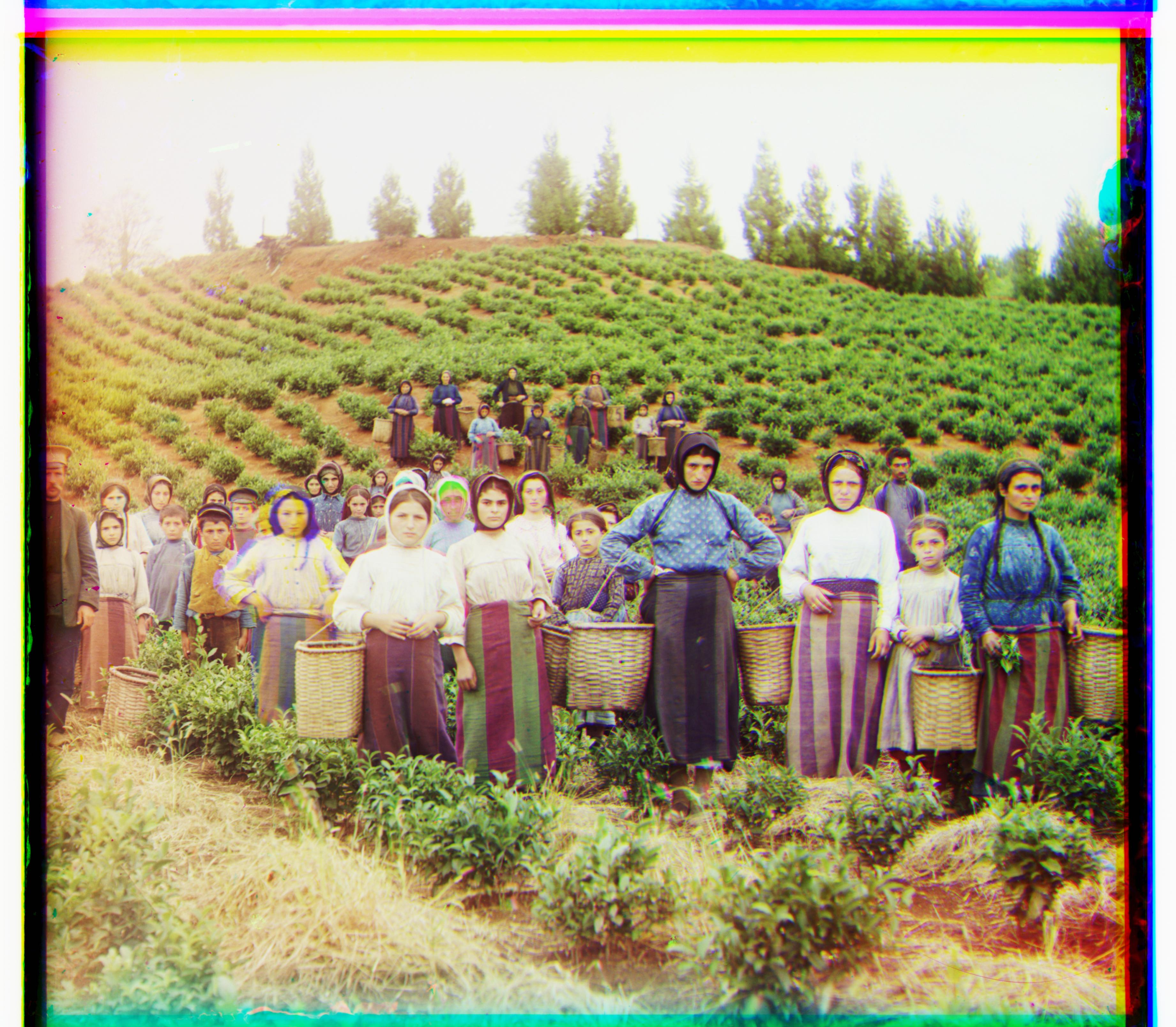
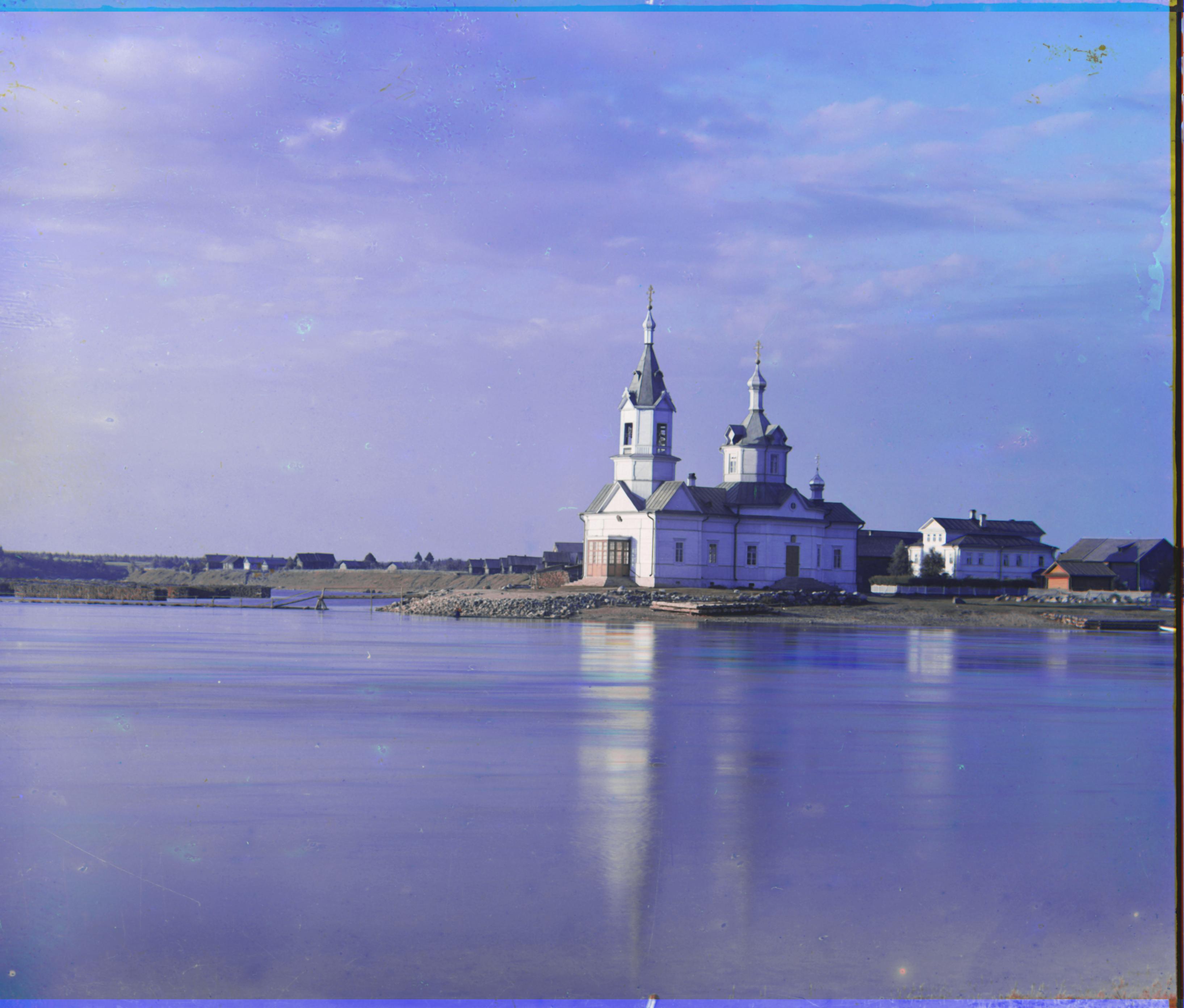
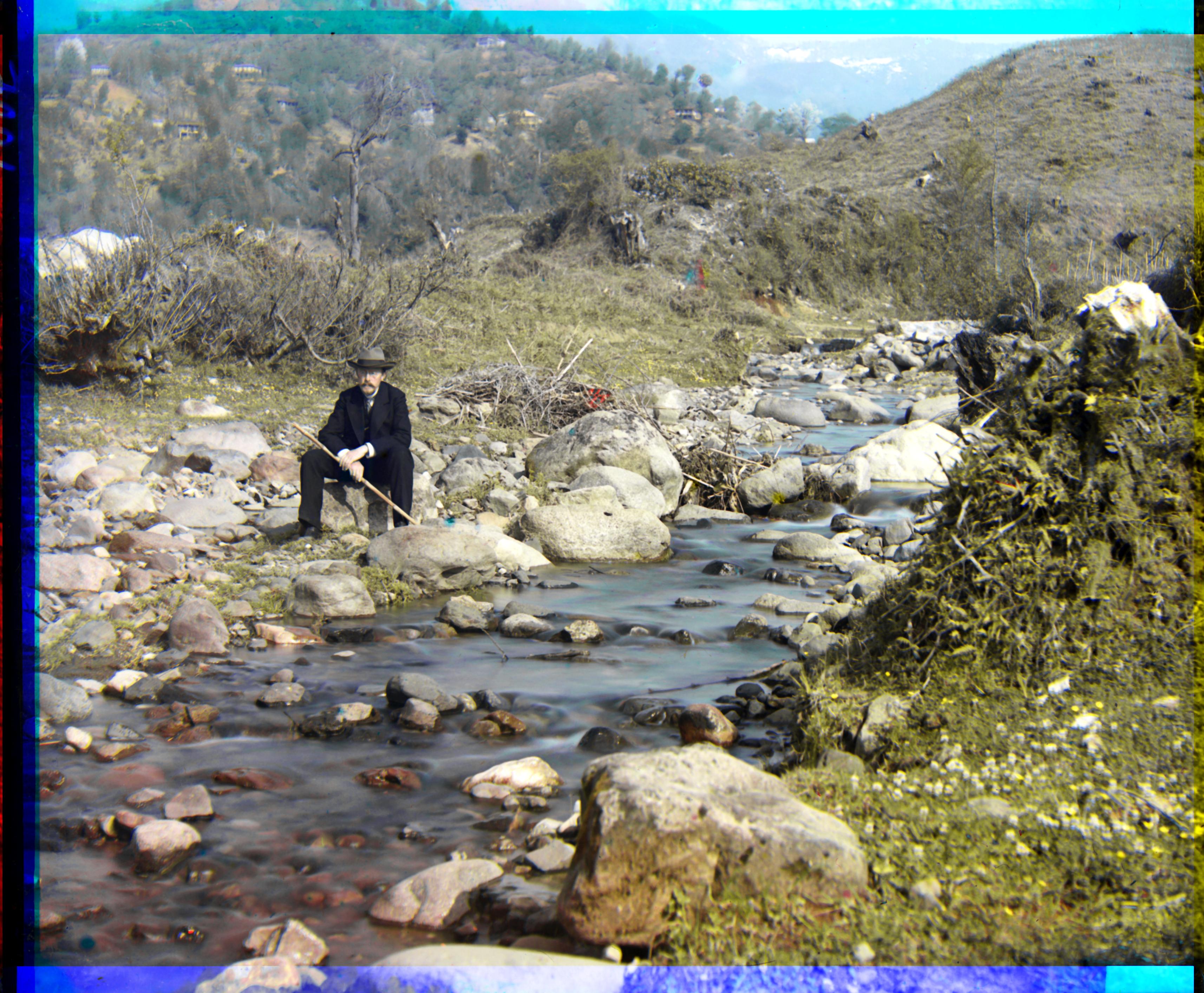
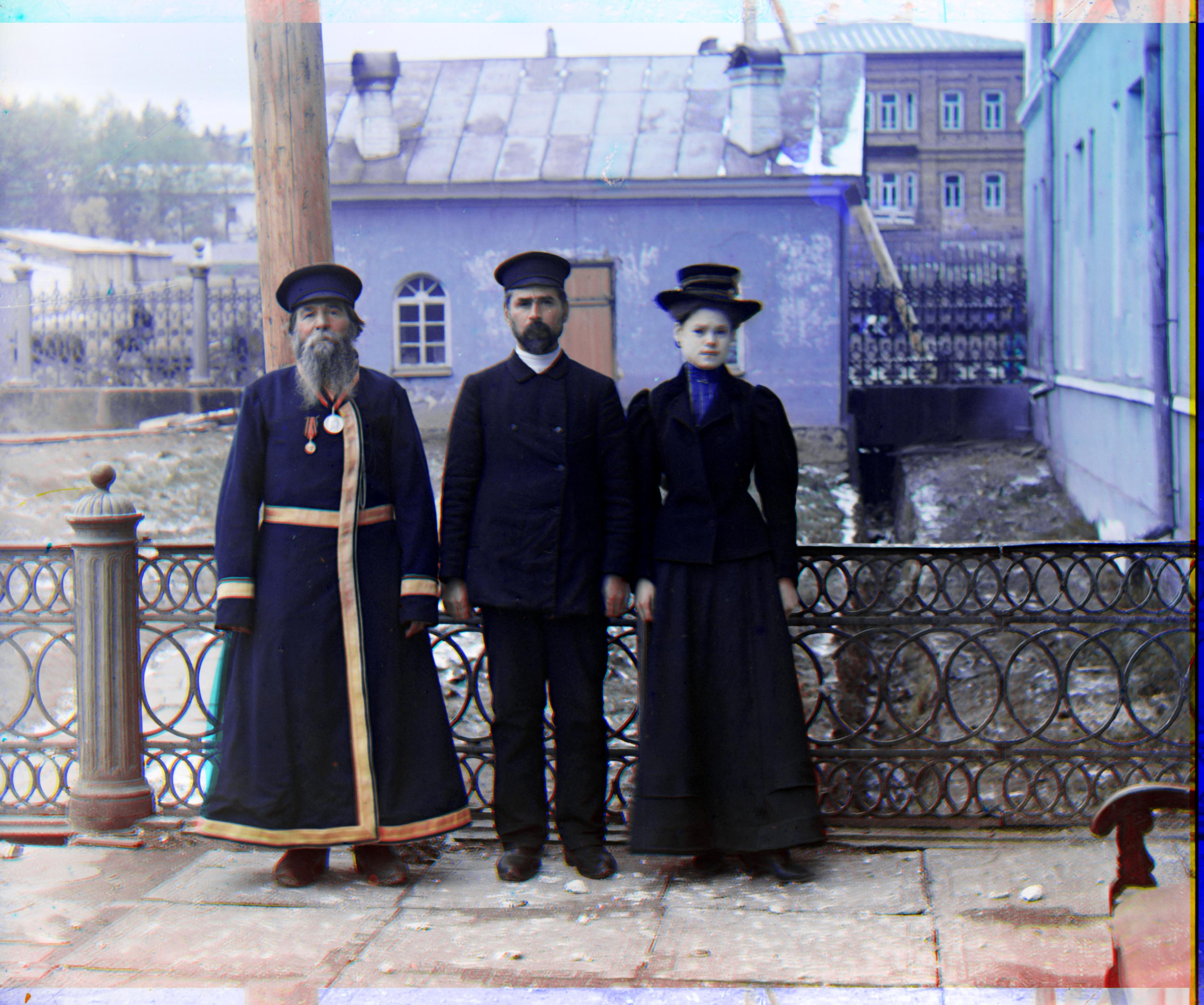
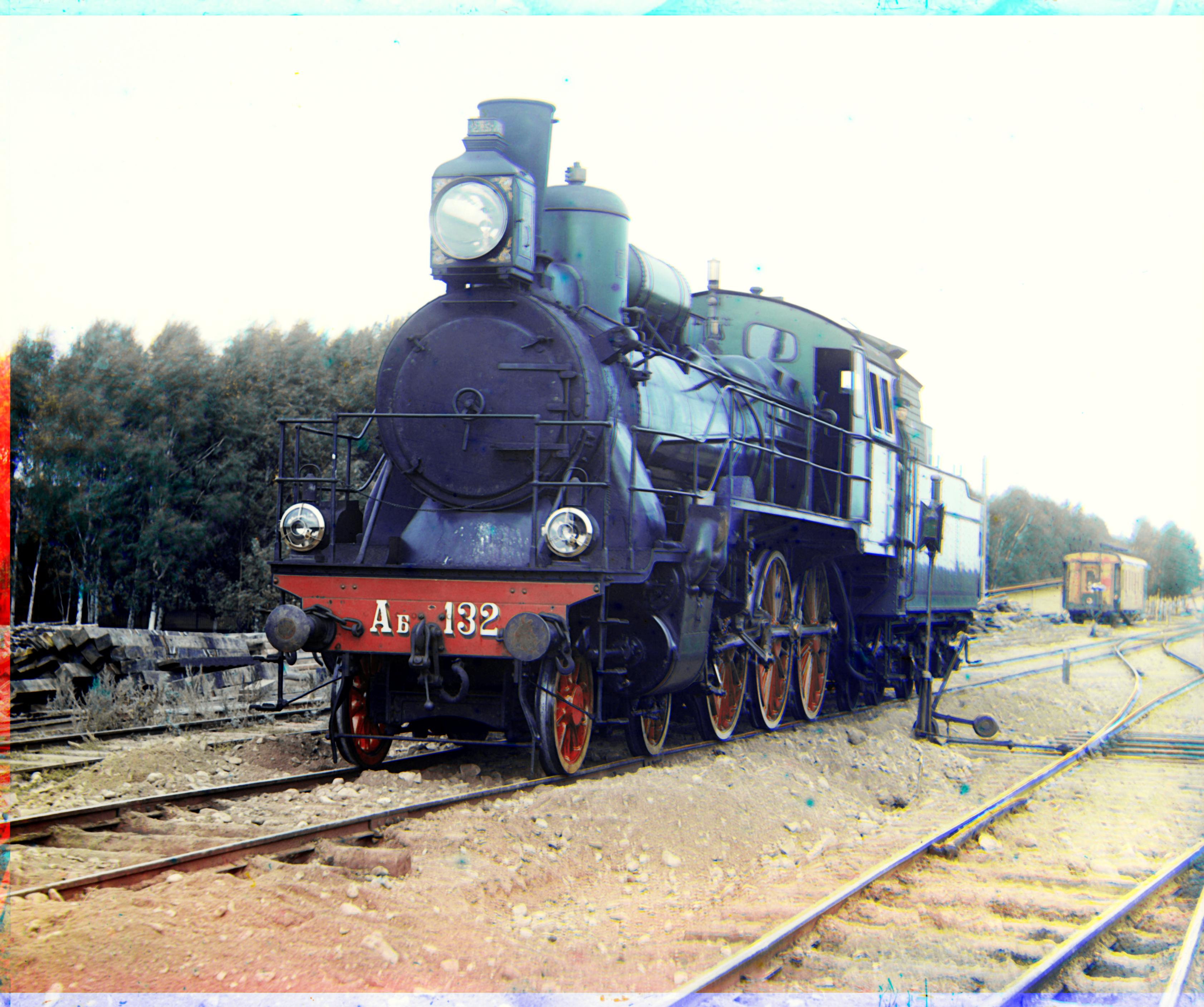
For this project, our objective was to create colored images from digitized Prokudin-Gorskii glass plate images using image processing techniques. In the following sections, I will detail my experience with the project and discuss the outcomes.

Initial Problem: Aligning The Images

Initially, to align the images, I followed the approach outlined in the project documentation, which suggested sliding the respective images within a defined space and calculating similarity metrics using various methods such as Euclidean distance and Normalized Cross Correlation. After reading through online course threads, I learned that many students had achieved great results using Mutual Information as their preferred metric. After implementing this approach, I found the results satisfactory. Consequently, I discovered a more innovative method, previously unknown to me, and decided to explore it.

Phase Cross Correlation - Bells & Whistles

Phase cross correlation shifts focus from searching for RGB similarities in the visual pixel domain to analyzing the frequency domain. In this approach, we compare the frequencies to detect similarities. Initially, I utilized a standard version of the function for testing. Satisfied with the results, I decided to implement an aligning algorithm, that aligns the initial images using phase cross correlation. After that, I decided to use the image sliding approach to fine-tune the results by applying image sliding on the initially aligned images. With this way, I was able to achieve satisfactory alignment results in great efficiency. Encouraged by this improvement and learning that it would be extra credit worthy, I delved into the algorithm's principles to understand and implement it myself as it was mentioned to be part of the B&W on Ed. Below, I have shared the custom function I coded, where I also explain the underlying logic.


        FB = fft2(base_image)
        F1 = fft2(image_1)
        F2 = fft2(image_2)

Finding the FFT of the images allows us to carry the images from the visual pixel domain to the frequency domain.


                    cross_power_spectrum_1 = (FB * np.conj(F1)) / np.abs(FB * np.conj(F1))
                    cross_power_spectrum_2 = (FB * np.conj(F2)) / np.abs(FB * np.conj(F2))

Calculating the cross power spectrum and normalizing the calculations are important because it enables us to access the phase differences between images, which is helpful because by this way, we eliminate the influence of intensities of pixels and focus on the geometrical composition of the images when searching for shifts.


                    correlation_1 = fftshift(ifft2(cross_power_spectrum_1))
                    correlation_2 = fftshift(ifft2(cross_power_spectrum_2))

When we take the cross power spectrums to the visual pixel domain back again by applying inverse FFT and shift the zero-frequency component to the center of the resulting matrix, we are essentially making it intuitively easier to find the peak from the correlation matrix by centering it from the corners.


                    maxloc_1 = np.unravel_index(np.argmax(np.abs(correlation_1)), correlation_1.shape)
                    maxloc_2 = np.unravel_index(np.argmax(np.abs(correlation_2)), correlation_2.shape)

Then, we search the matrices for the peak in order to find the information for the correct shift to align the images.


                    shift_x1 = maxloc_1[1] - base_image.shape[1] // 2
                    shift_y1 = maxloc_1[0] - base_image.shape[0] // 2
                    shift_x2 = maxloc_2[1] - base_image.shape[1] // 2
                    shift_y2 = maxloc_2[0] - base_image.shape[0] // 2

The purpose of the fftshift becomes clearer as we subtract the center of the image from the peak coordinates to find the pixel shifts for aligning the images.

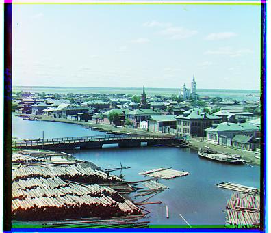
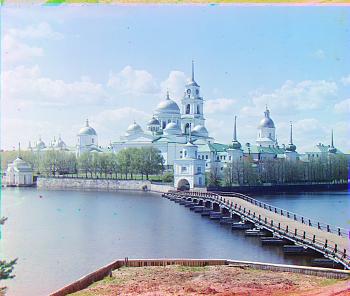
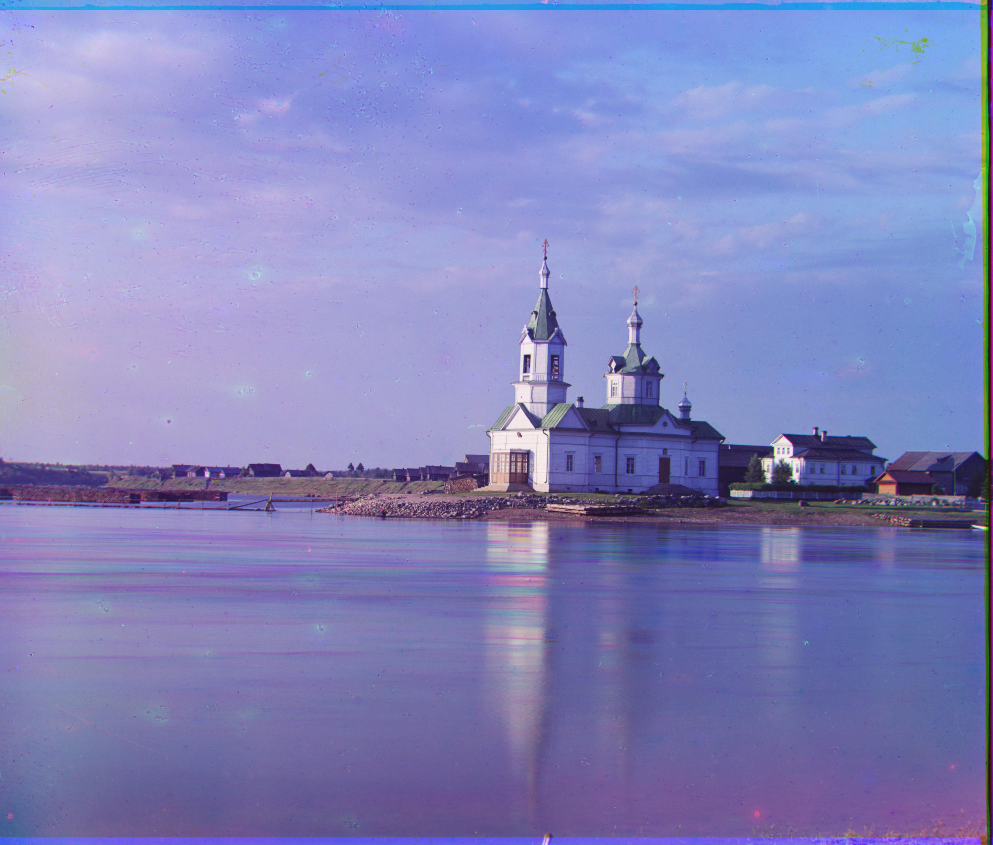
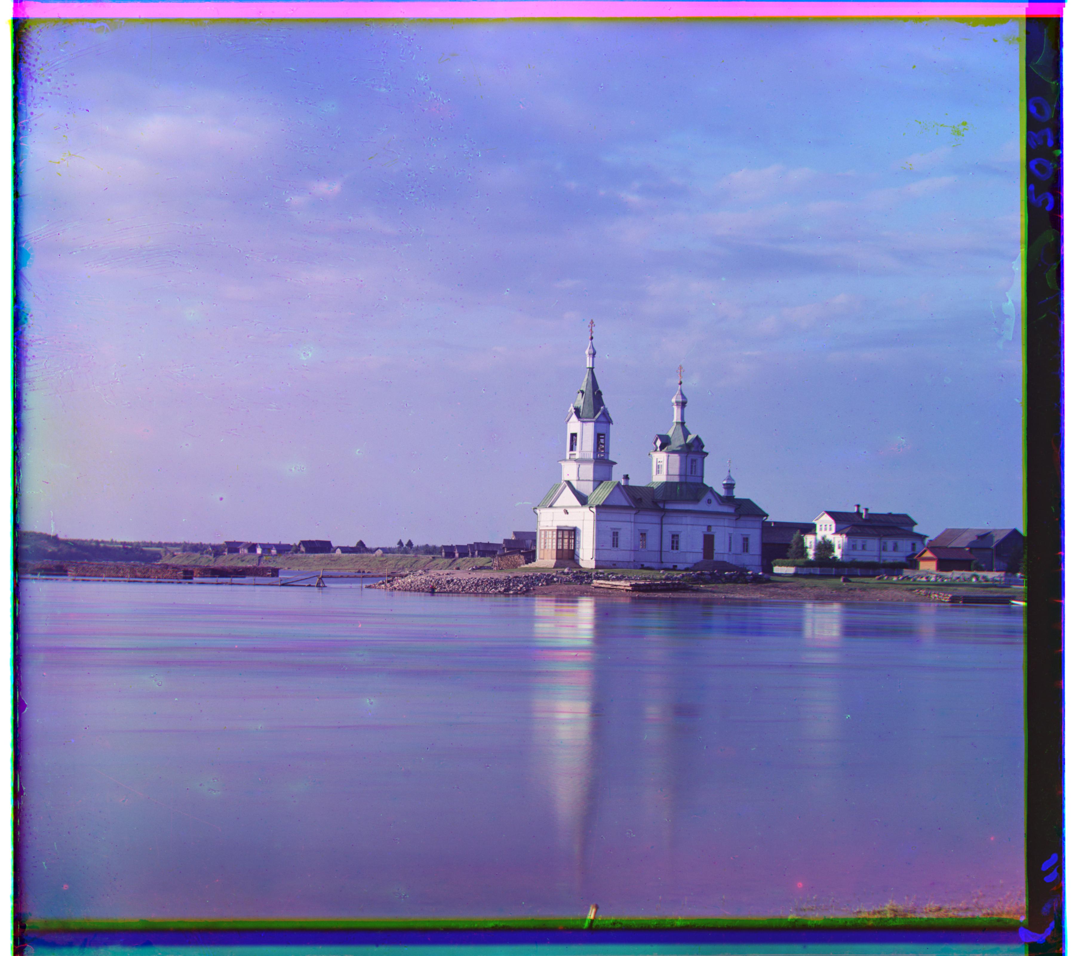
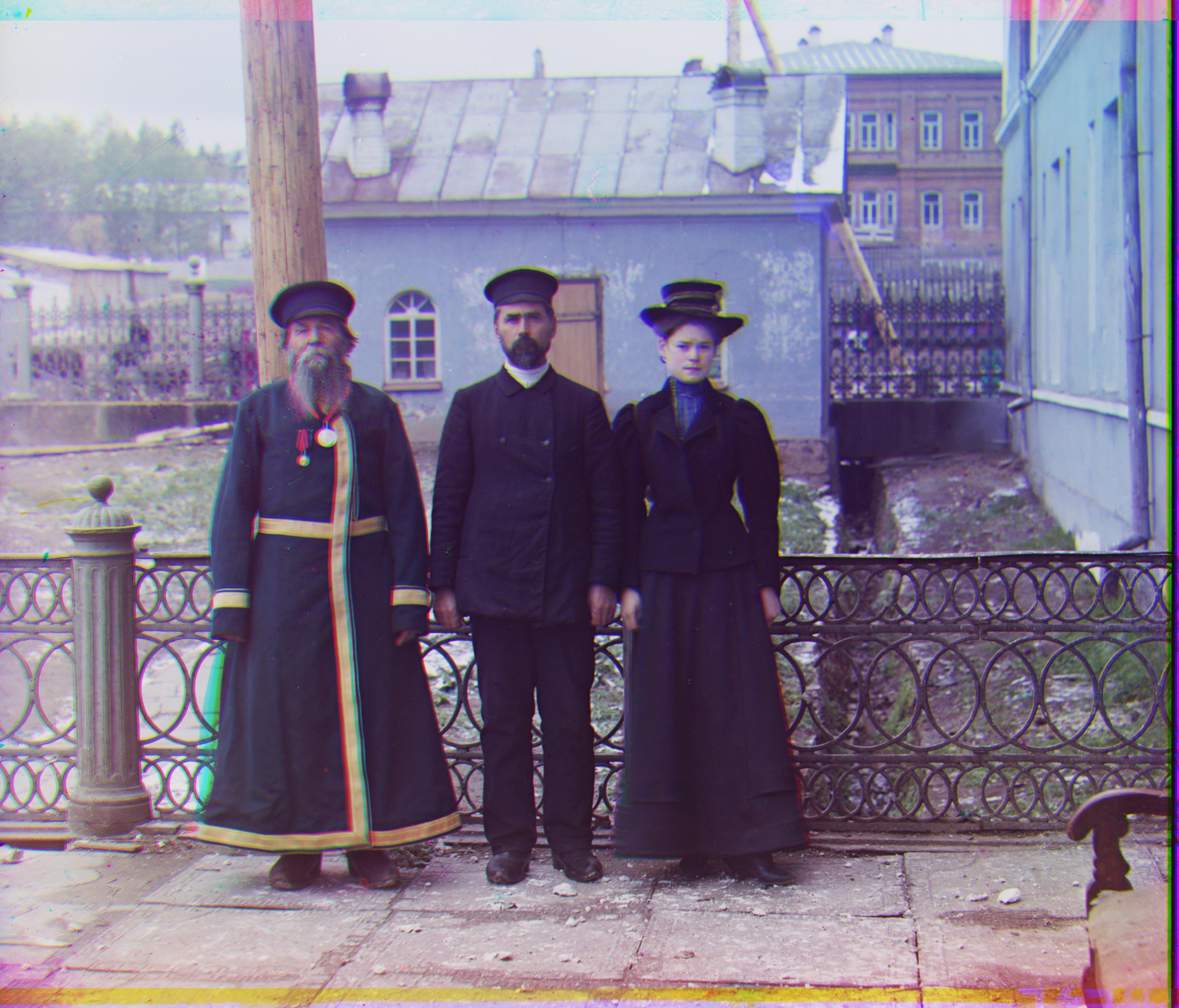
Here are a couple of the results:

Although not terrible, you can see the presence of the borders and one can intuitively tell that it would make it harder to align the pictures as borders aren't consistent. Therefore, I decided to crop the borders. I have used automatic border cropping algorithms but I have only seen success with them for removing the white border on the outside, but not the darker ones surrounding the image content. Therefore, I decided to get the center 90% of the image and discard the rest in the corners. However, after testing with this setup, top of the images still had flares due to borders so I decided to cut additional 3% from the top of the image, making me crop 8% from the top and 5% from the rest of the sides.

Here are the results after cropping and changing the alignment base to G as testing empirically I had better results:

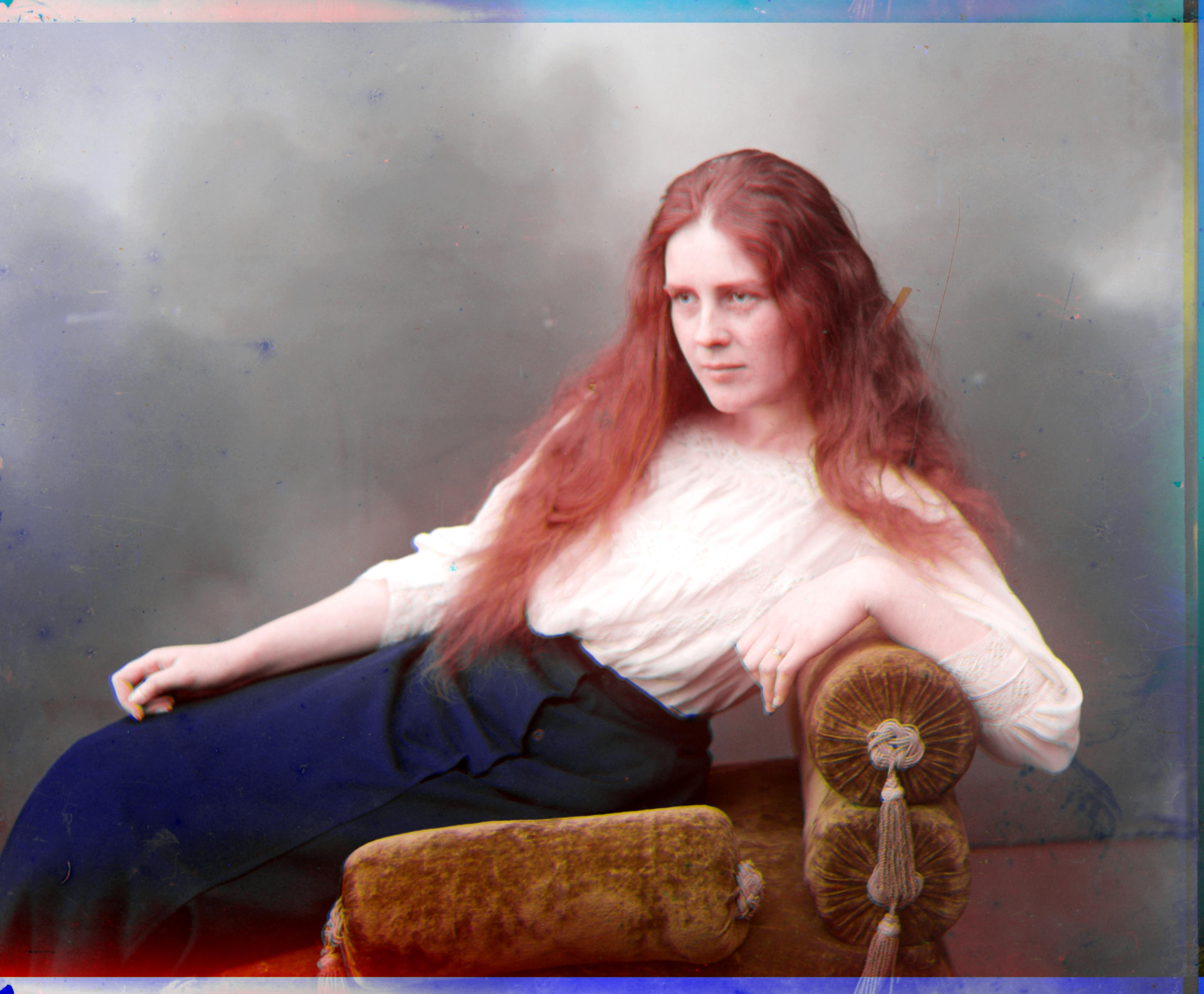
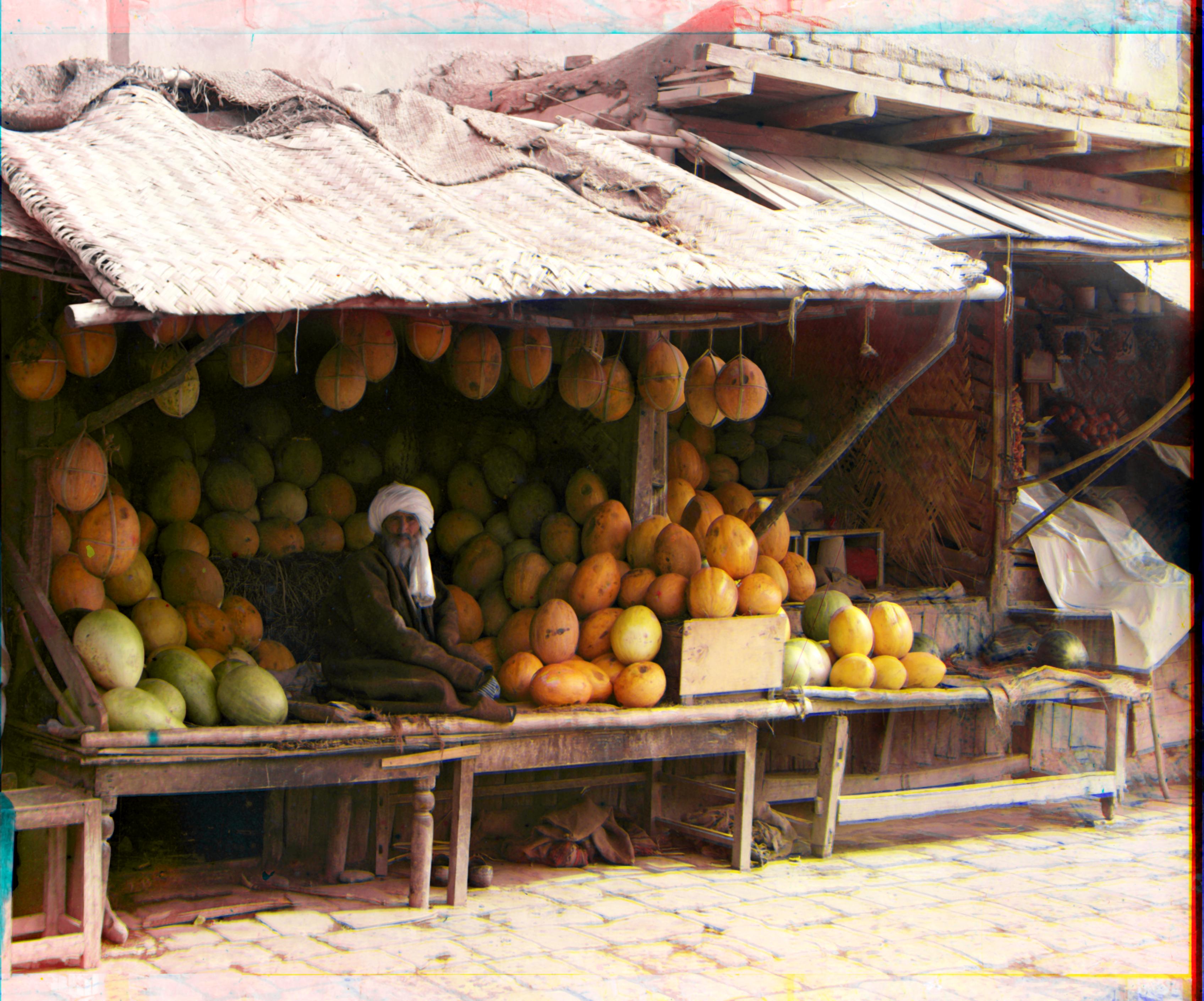
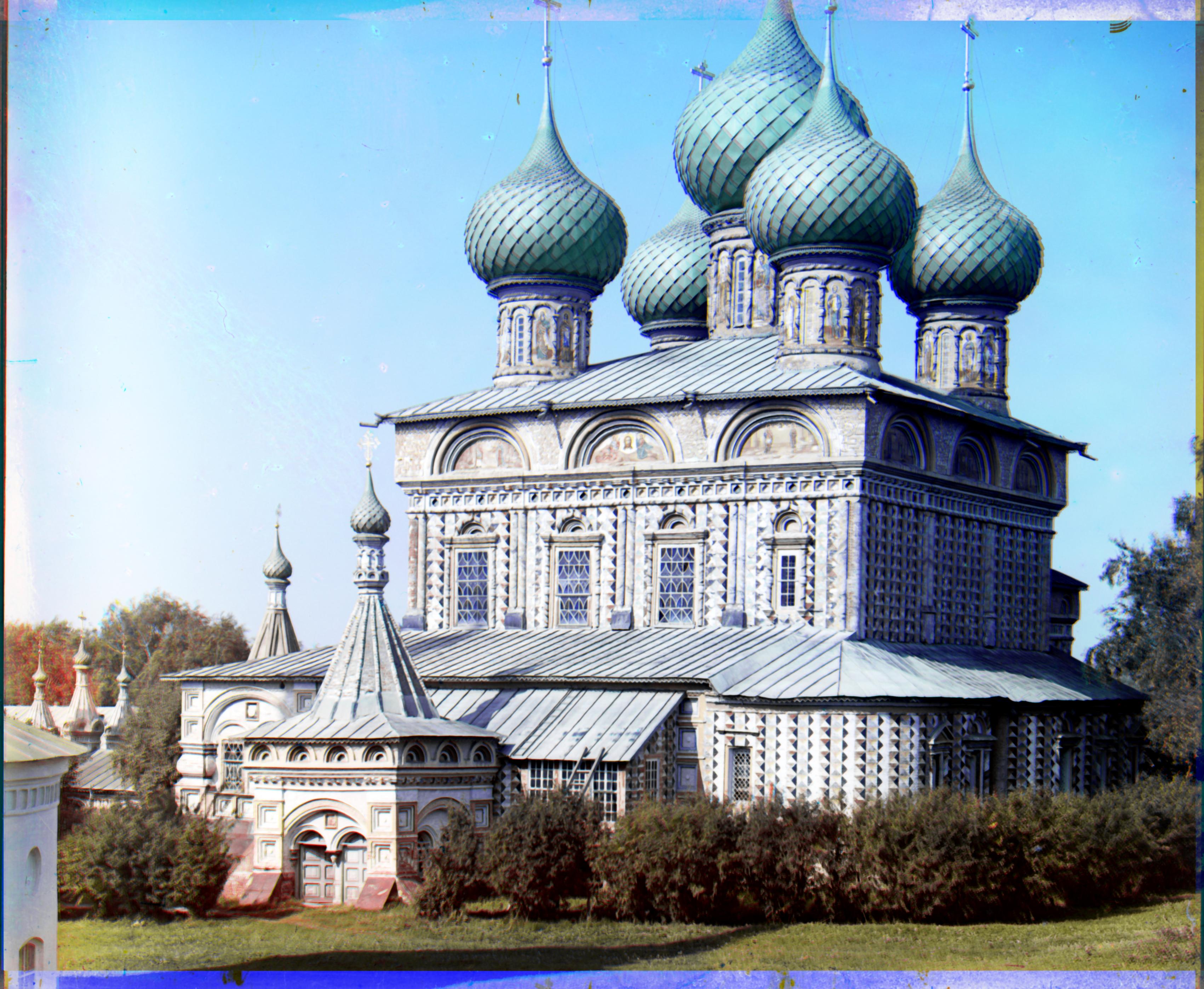
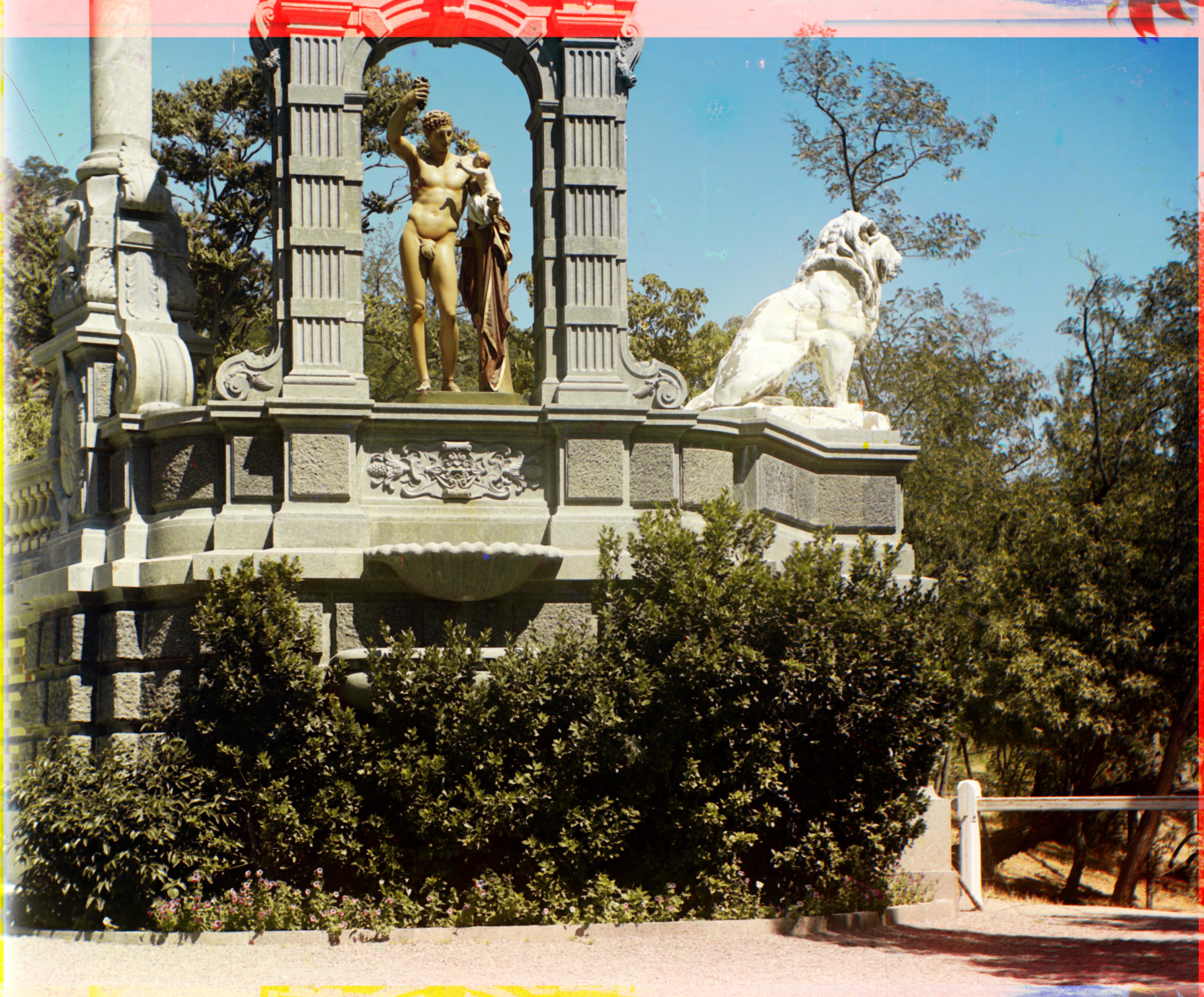
However, this approach worked for the smaller resolution images. For the larger .tif images, I had to implement a coarse-to-fine pyramid speedup for alignment algorithms. I decided to use 4 layers as I saw great results without major speed drawbacks. As to the system of the pyramid speedup, I build a pyramid with coarse to finer resolution images of our base image. Then, I start consuming from the coarsest one and calculate the alignments as I step through the layers of the pyramid. The alignment logic stays the same: phase cross correlation for the initial alignment, then I slide the images over the base image for fine tuning the alignments. Since I apply the shift's at each level while keeping track of the cumulative shift which is the multiplication of the previous shifts with 2 as the resolution increases to twice the size with each step. Here are the results on larger resolution images:

Additional Image Enhancements - Bells & Whistles?

Curious how far I could push the results from the images, I explored what else could be applied to the pictures. Noticing that a good portion of the images had really small distortions, marks, inconsistencies, and etc. I decided to apply a median filter over the image, to smooth out these errors.

Thinking that removing the small distortions over the image would help more if done before stretching the contrast of the image in order to not scale up the distortions as well, I decided to stretch the contrast of the image, which basically stretches the middle-ranged pixel values to both ends of the spectrum. This would give the image more contrast, and make it sharper.

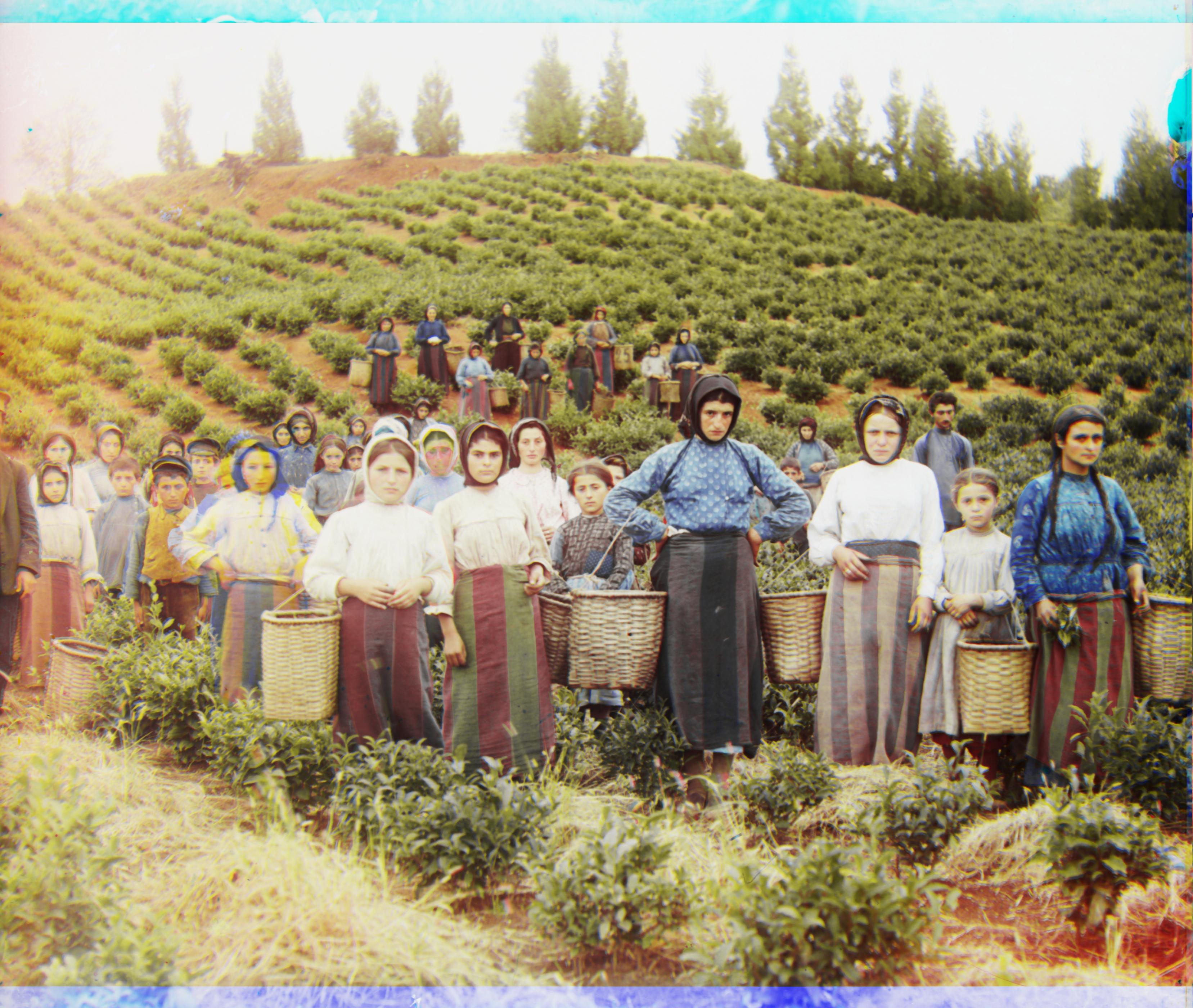
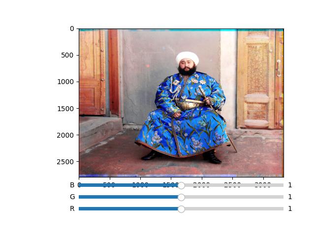
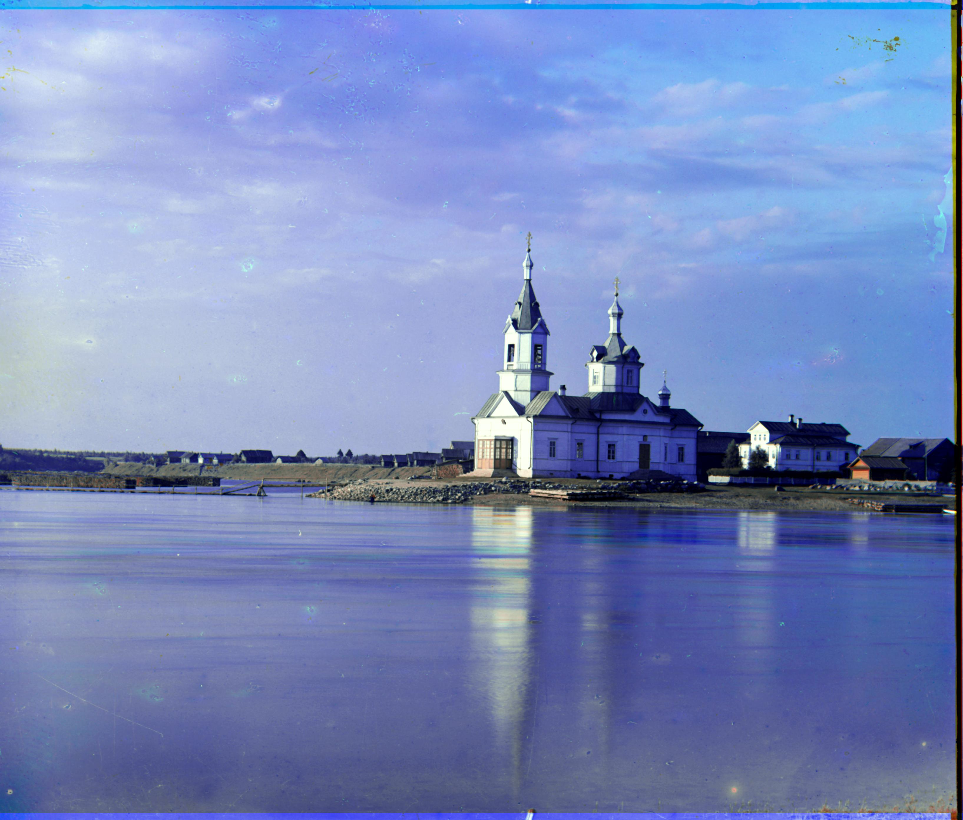
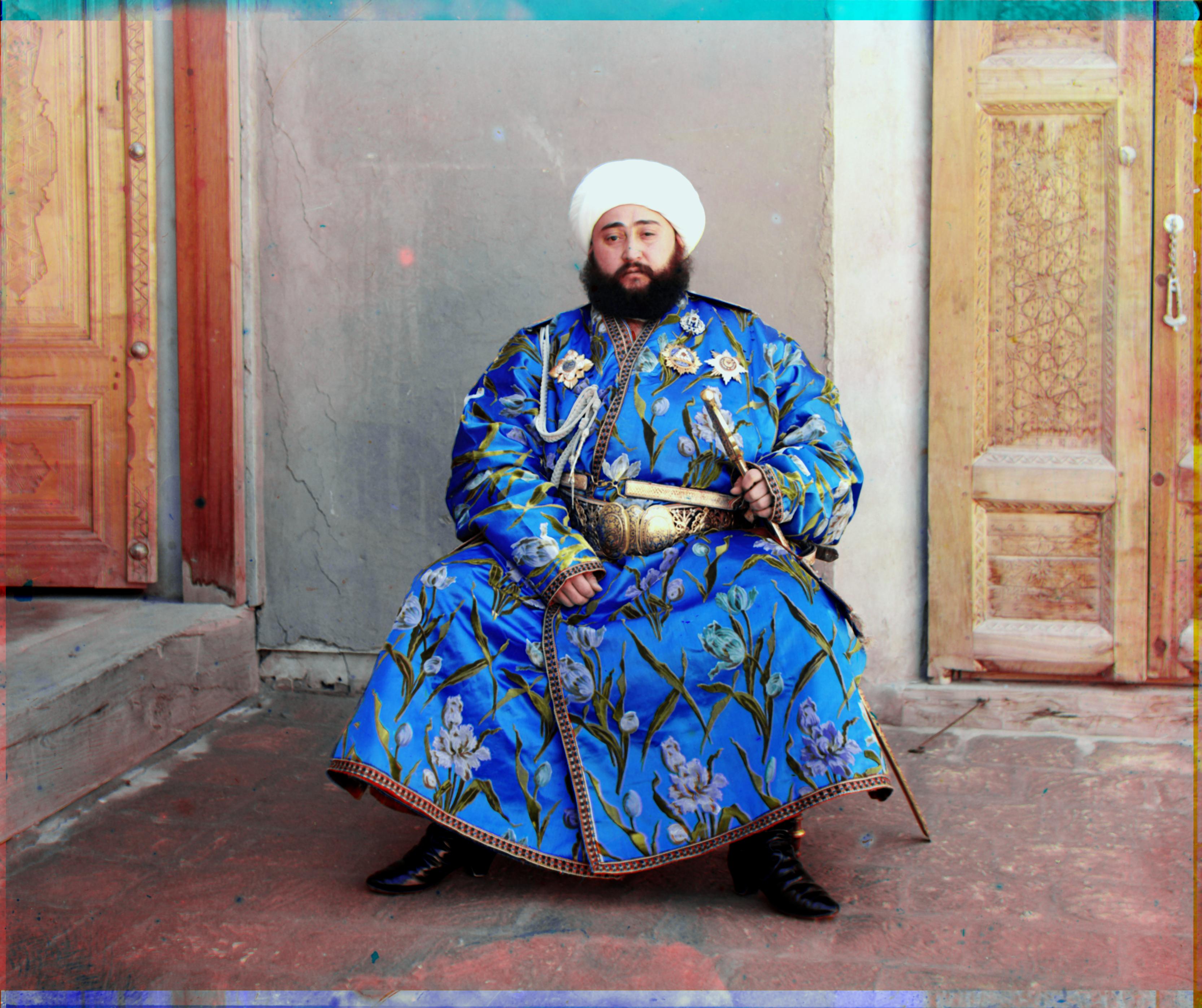
Finally, since unfortunately I got lazy to implement further automatic contrasting techniques, I built this tool with the following UI to manually tweak the R,G,B intensities to apply color adjustments to add the final touch personally. Here are the last version of all the images with their respective shifts: