CS180 Final Project: Facial Keypoint Detection with Neural Networks
Deniz Demirtas - Tan Sarp Gerzile
In this project, we are going to delve into the fundamental operating principles of diffusion models, and understand how does image generation with diffusion models work under the hood. To start off with, we are going to start with the DeepFloyd IF diffusion model. You can find more information about the model here.
Nose Tip Detection
To start, we are going to train a "toy" model using the IMM Face Database for nose tip detection. We are going to cast the nose detection problem as a pixel coordinate regression problem.
The CNN model we are going to start with is a simple 3 convolutional layer network with 16, 32, and 32 hidden layers for each. Each convolutional layer is followed by a ReLU activation function and then a max pooling layer. Then, the model is followed by 2 fully connected layers with 58 and 2 hidden units respectively, where the first layer is followed by a ReLU activation function. For training, we are going to use the Adam optimizer with a learning rate of 1e-3.
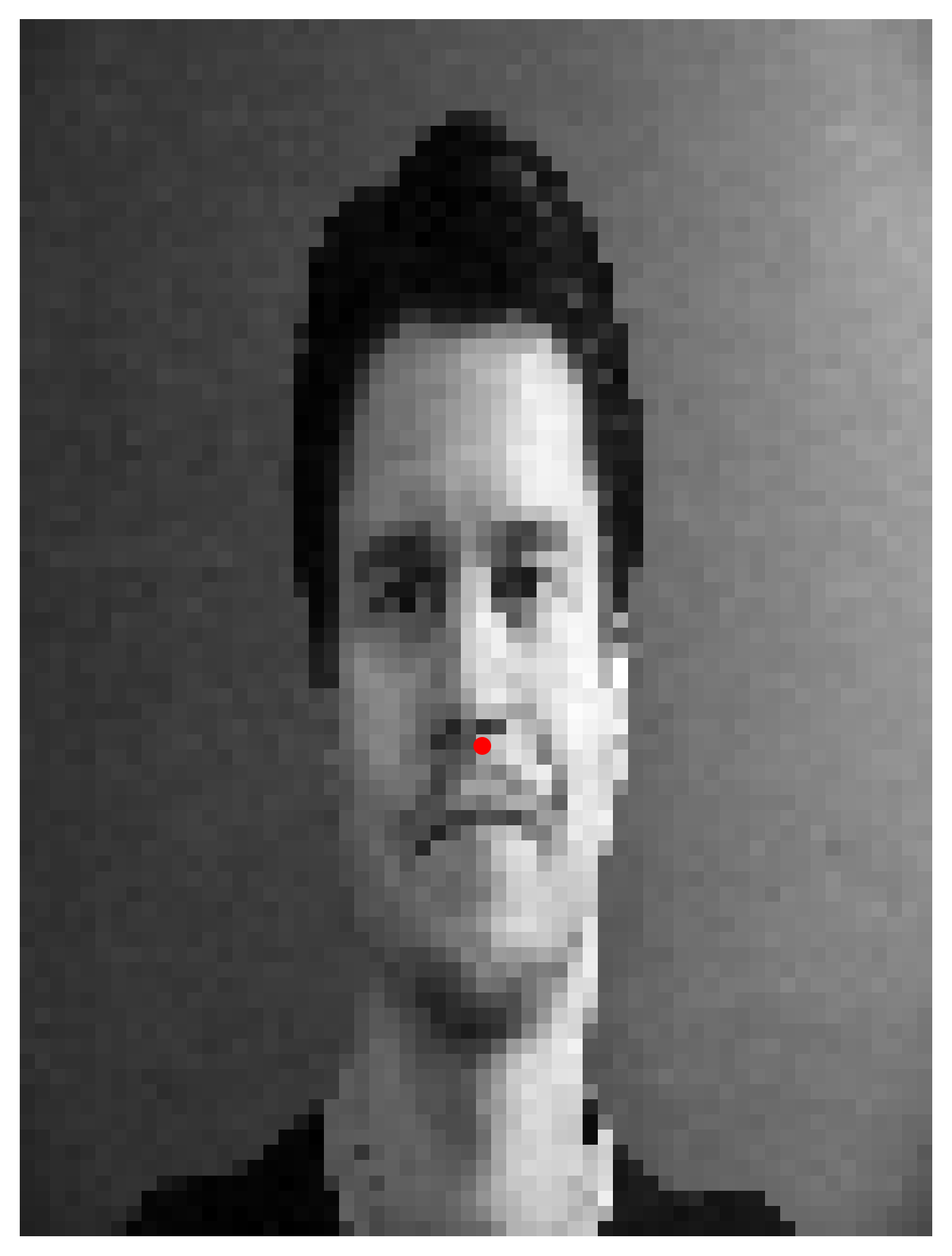
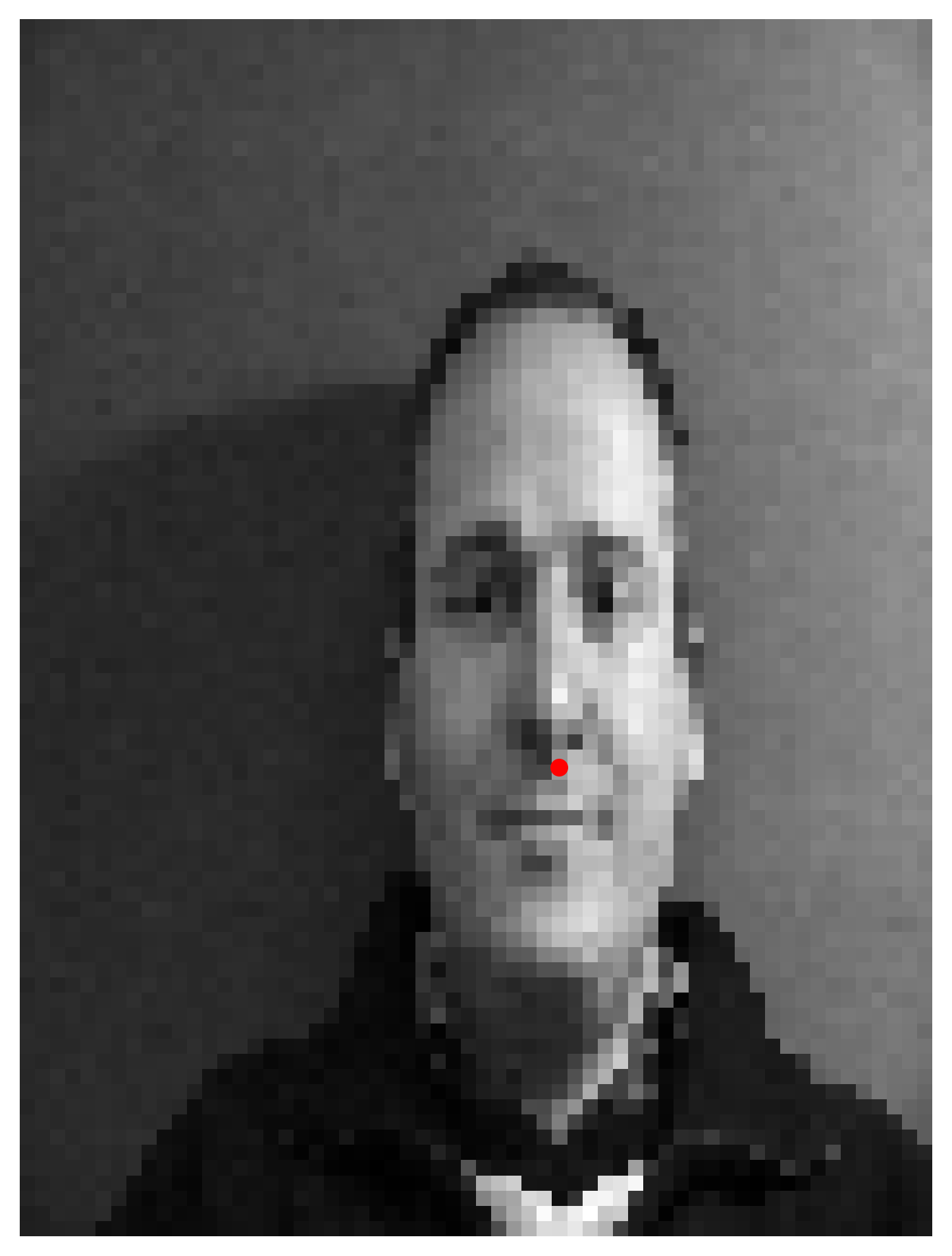
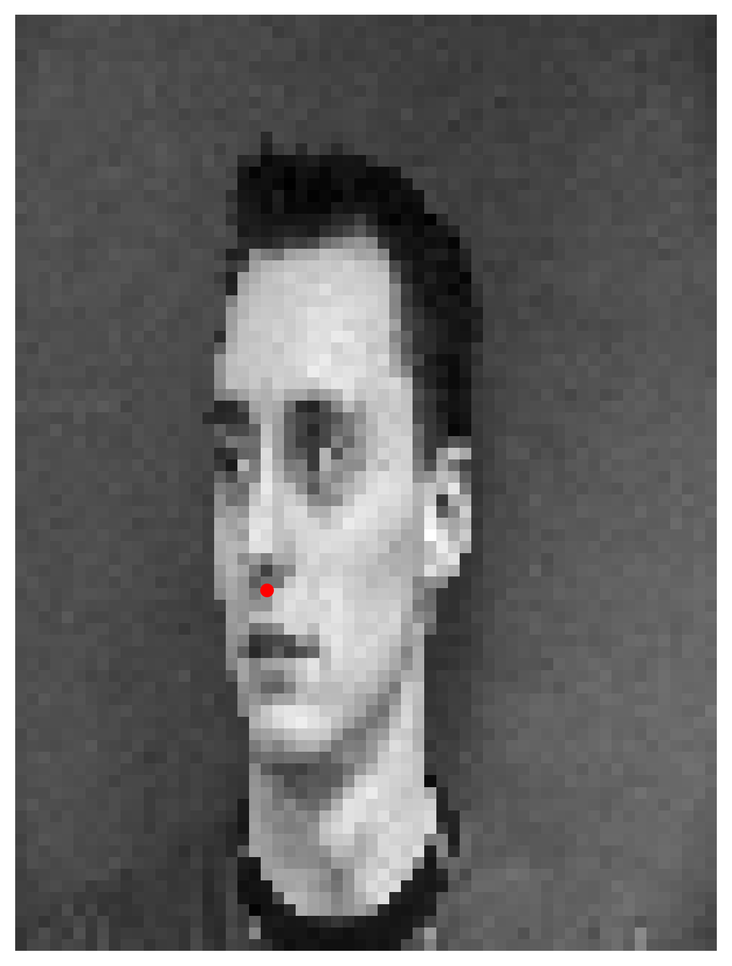
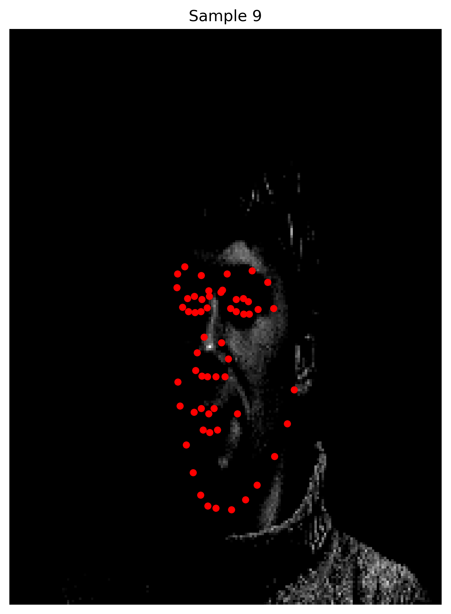
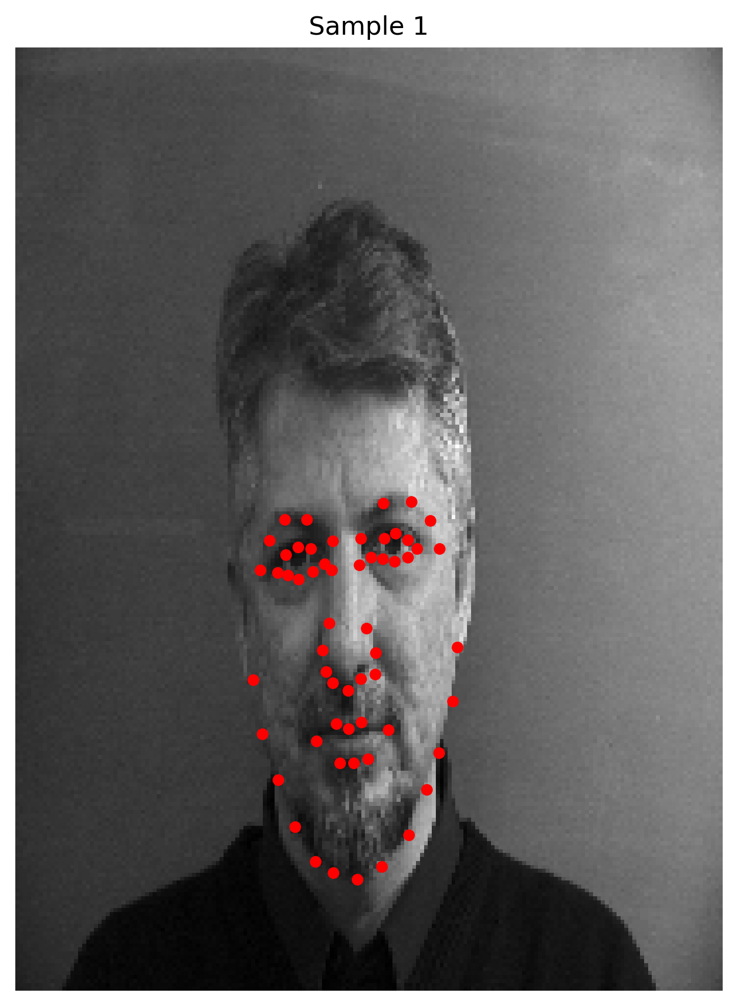
As for preparing the data, we load the images into grayscale, then normalize by converting the input data that's in uint8 [0, 255] to np.float32, in which they are centered around [-0.5, 0.5]. Here are some examples after initial processing with the landmark annotations for nose tips.
Images sampled from the training dataset after processing
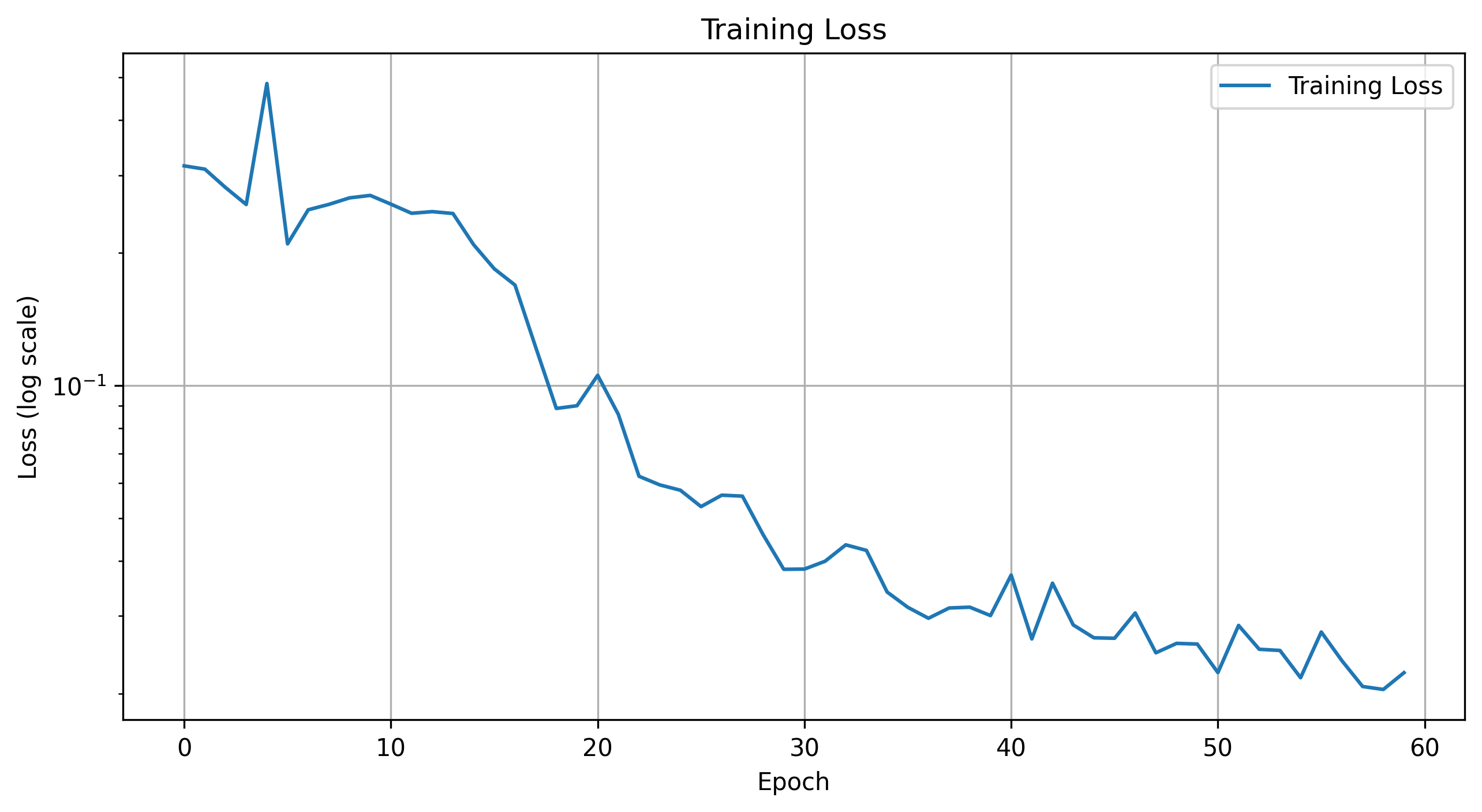
Here are the training and validation losses for the explained model for 10, 15, 20, and 25 epochs.
Training Loss
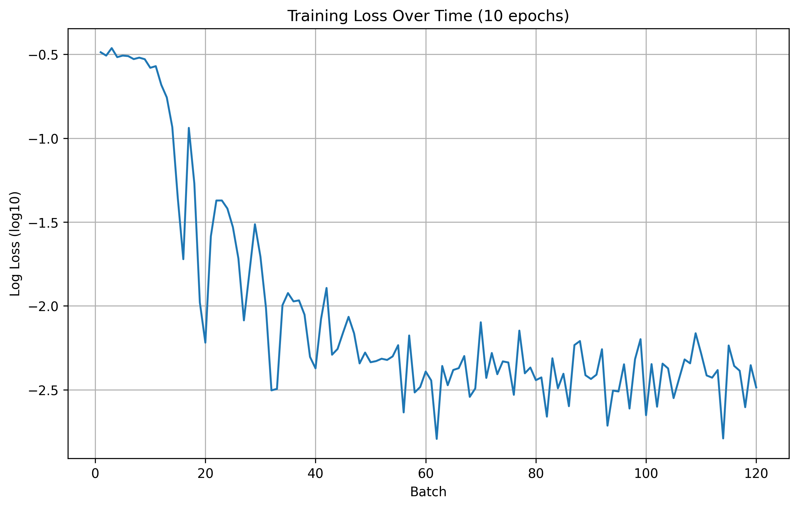
10 Epoch Training Loss
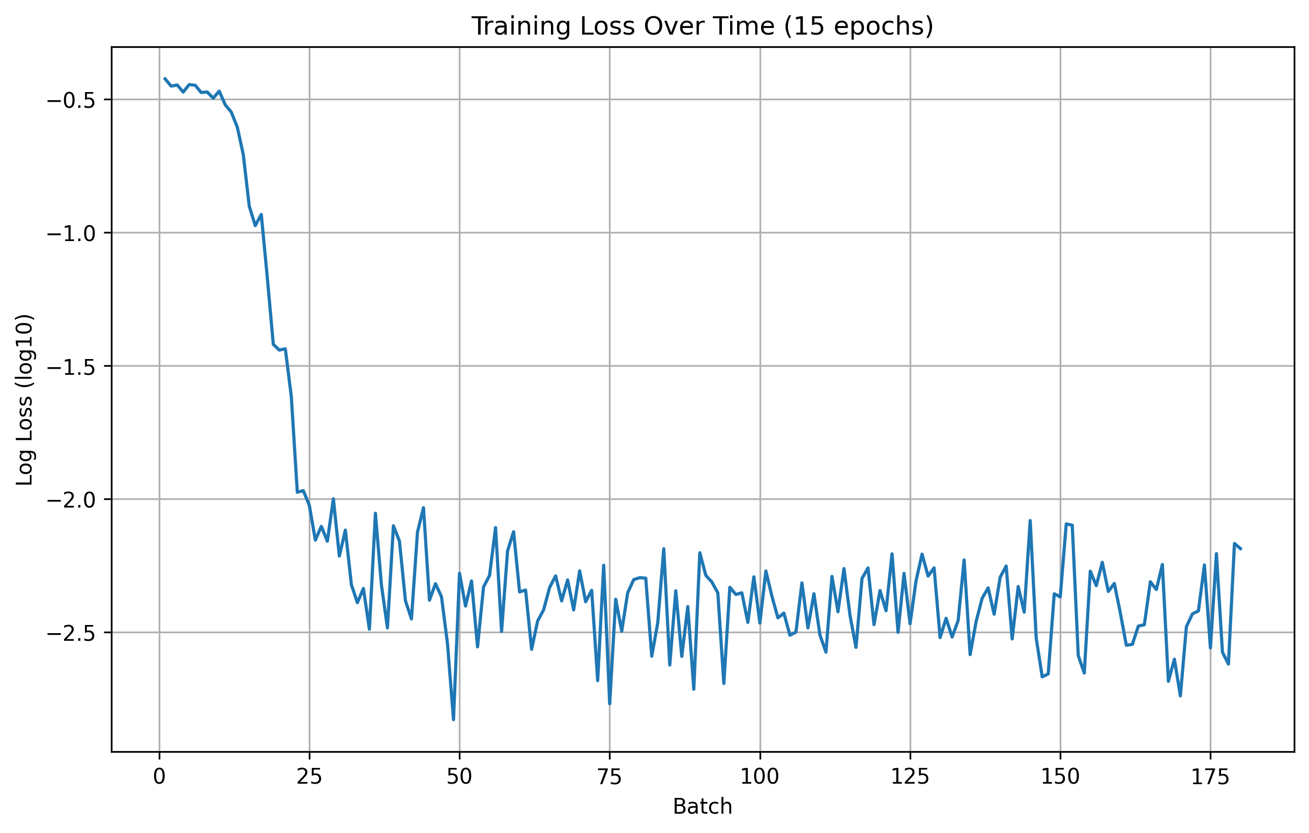
15 Epoch Training Loss
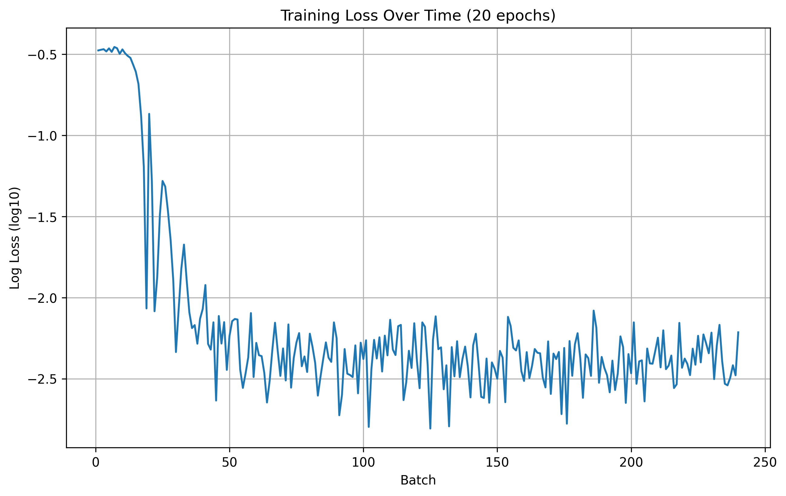
20 Epoch Training Loss
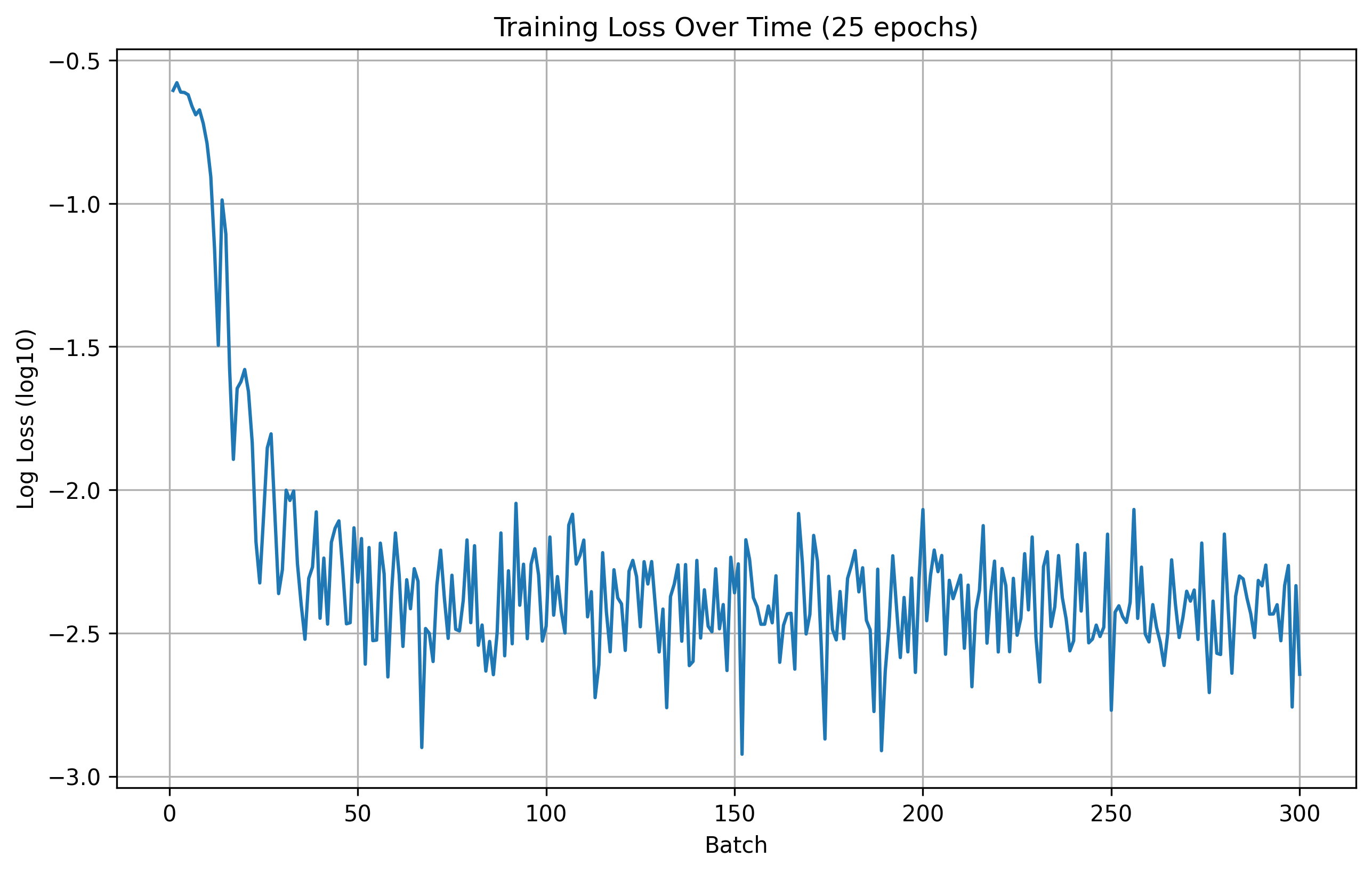
25 Epoch Training Loss
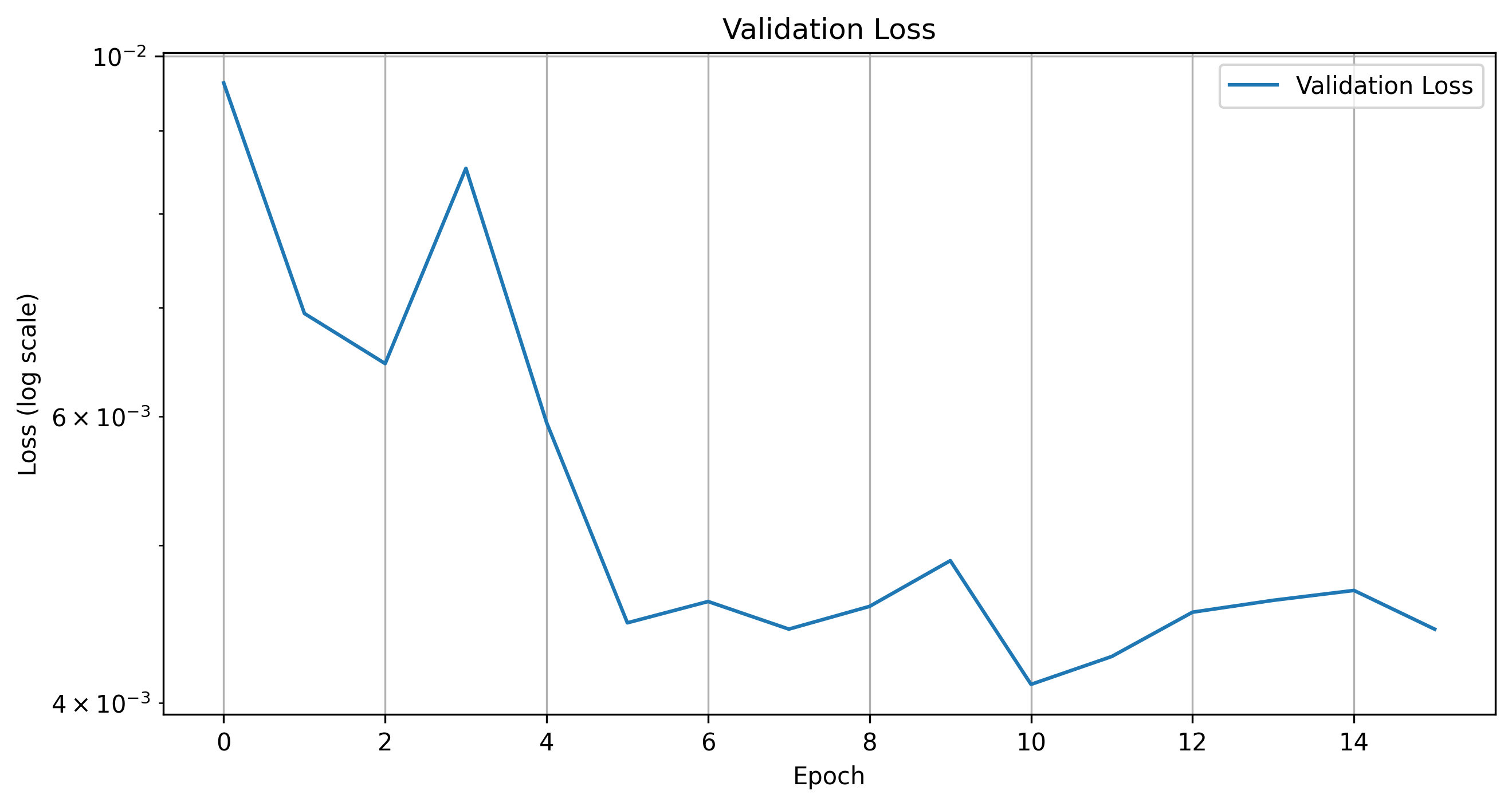
Validation Loss
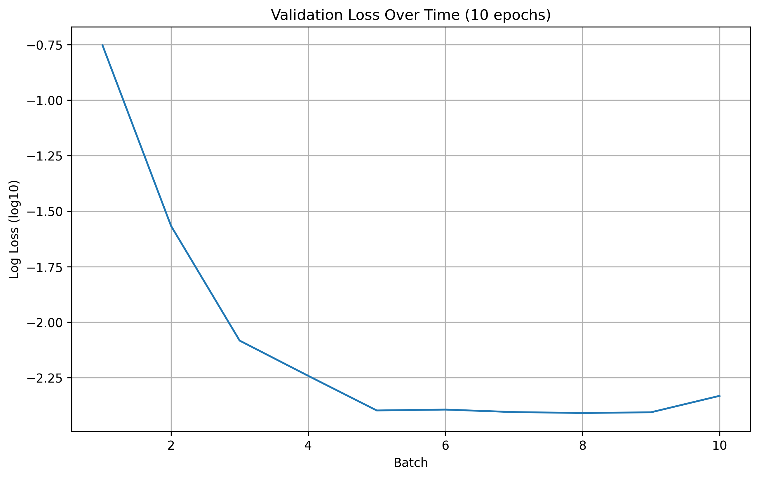
10 Epoch Validation Loss
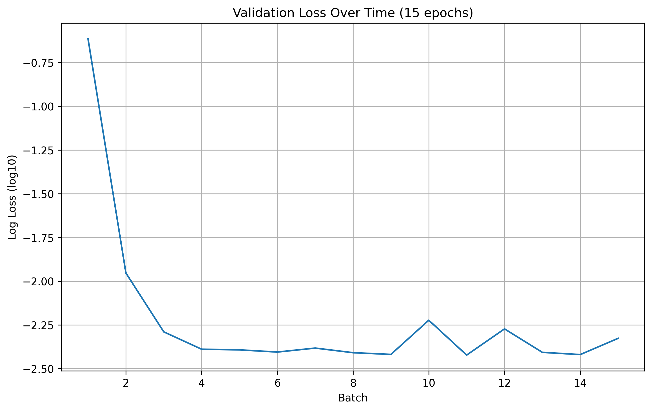
15 Epoch Validation Loss
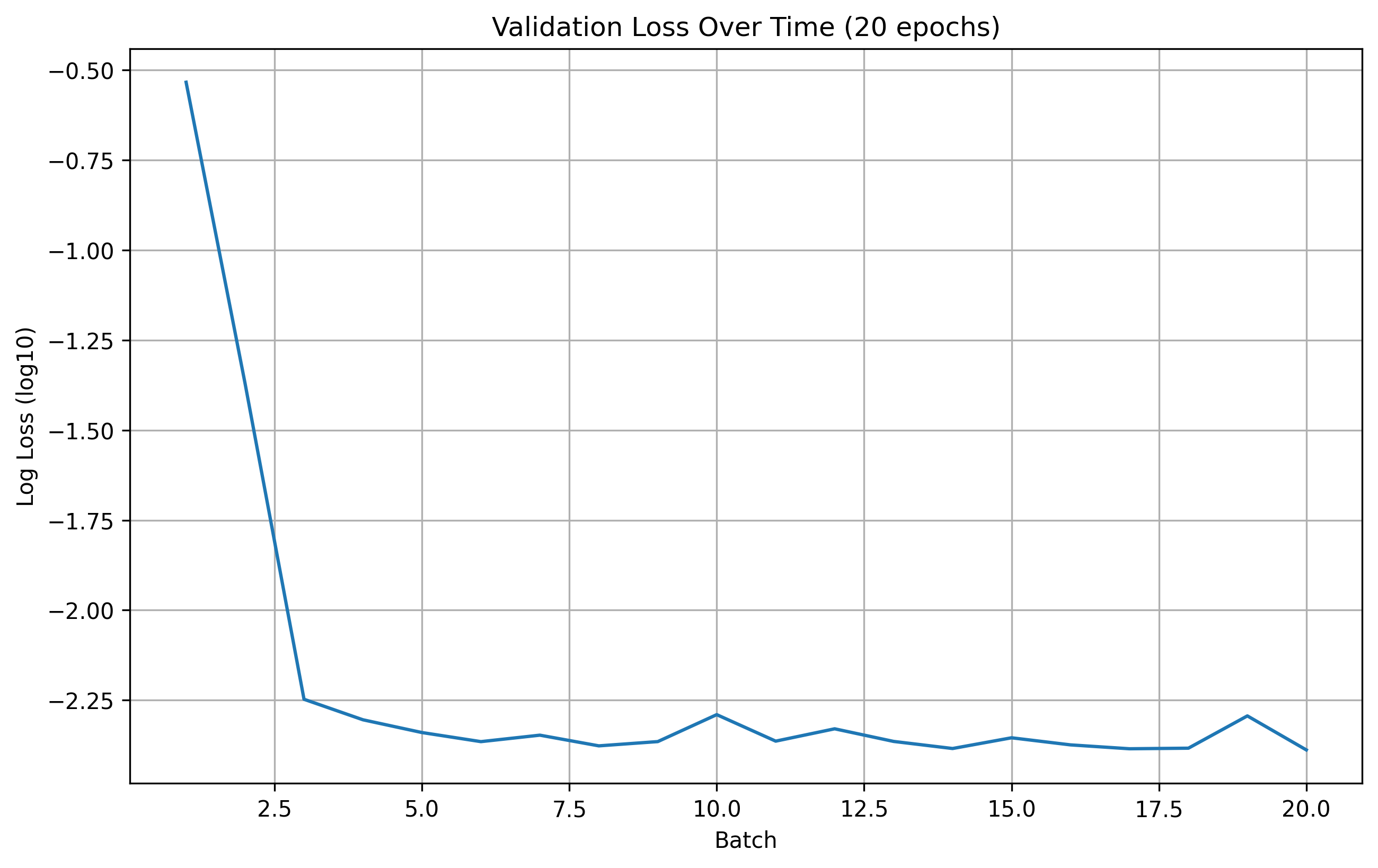
20 Epoch Validation Loss
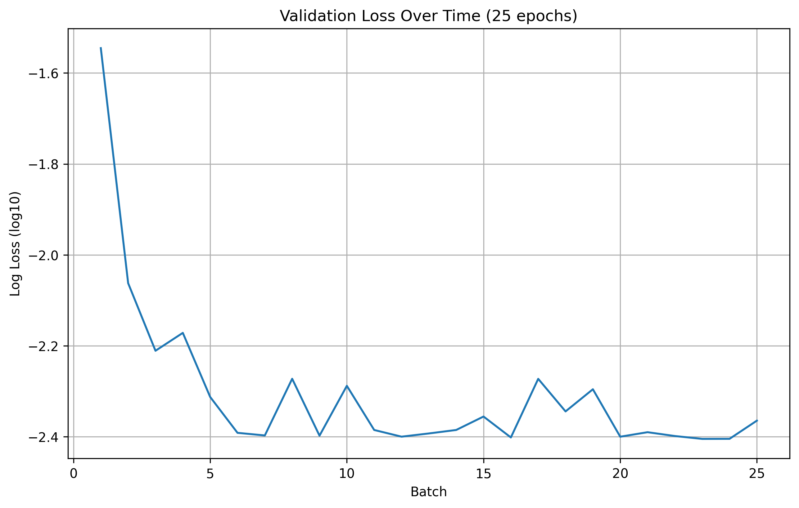
25 Epoch Validation Loss
From the results, we can see that the number of epochs don't offer a significant improvement in the model's performance. Therefore, for this part, we are going to use 20 epochs for training during hyperparameter search.
Here are some predictions from the model.
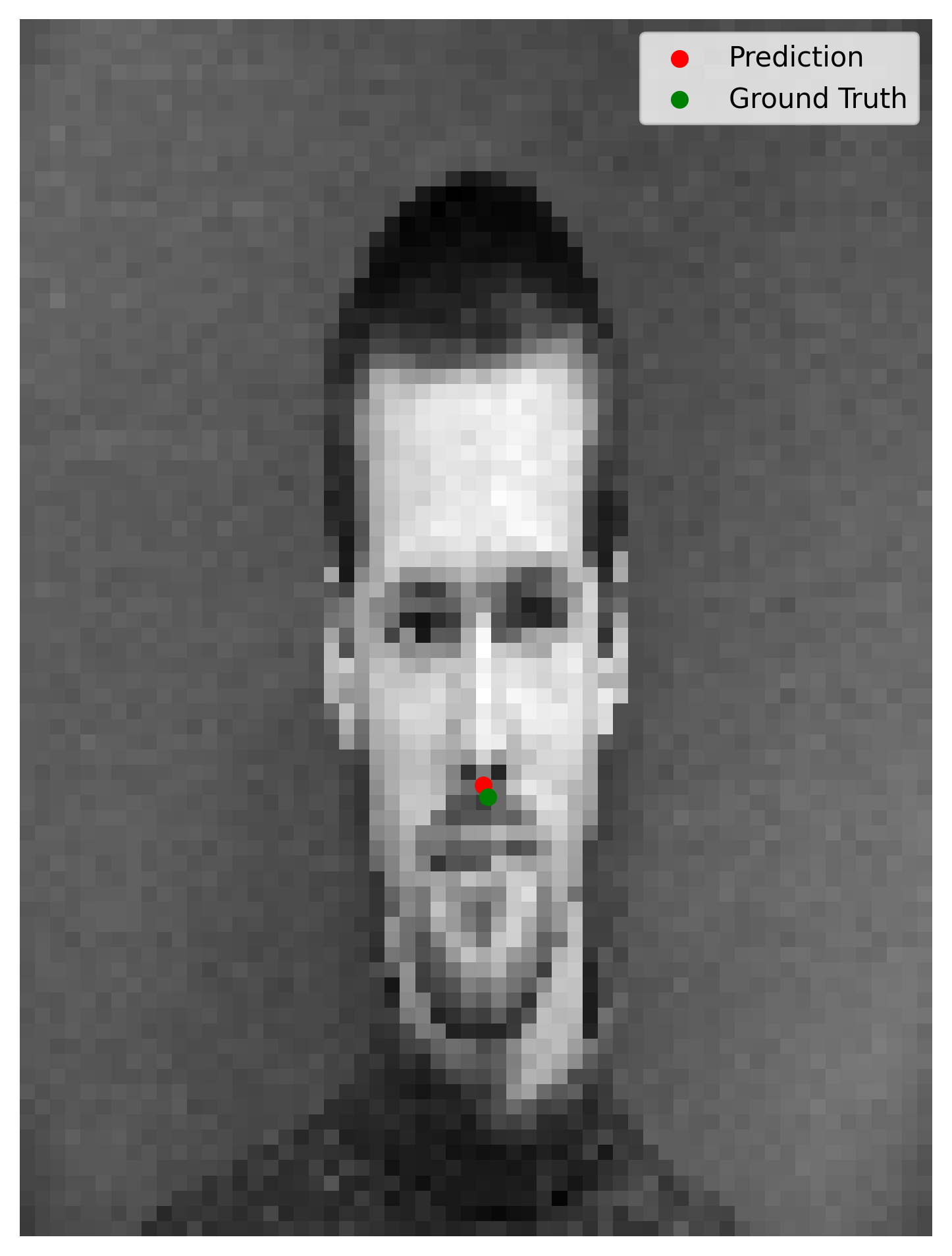
Prediction 0 (accurate)
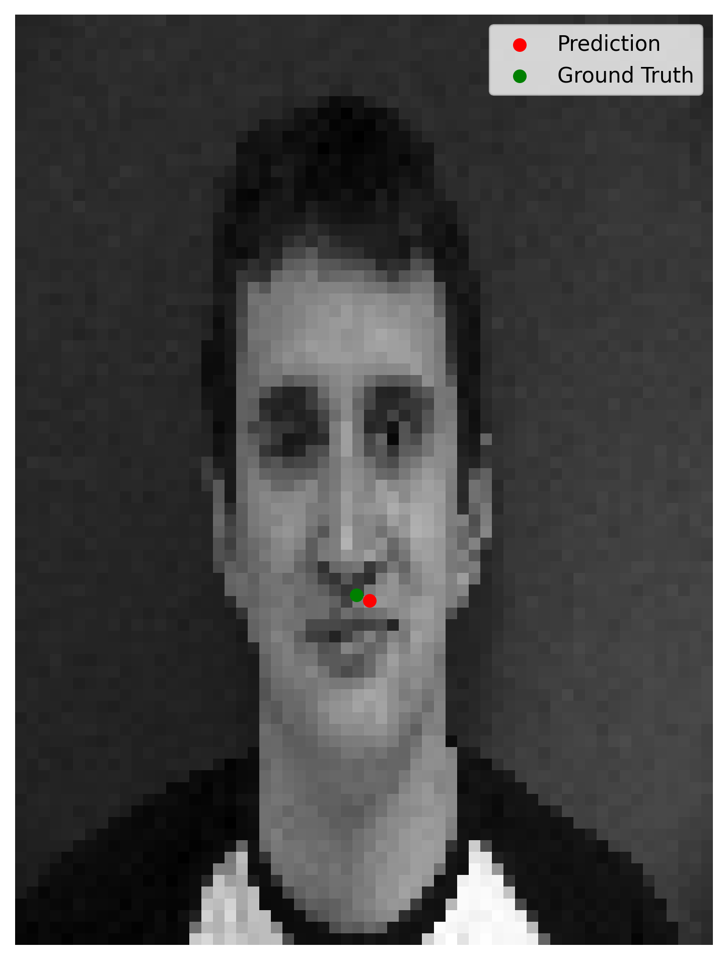
Prediction 1 (accurate)
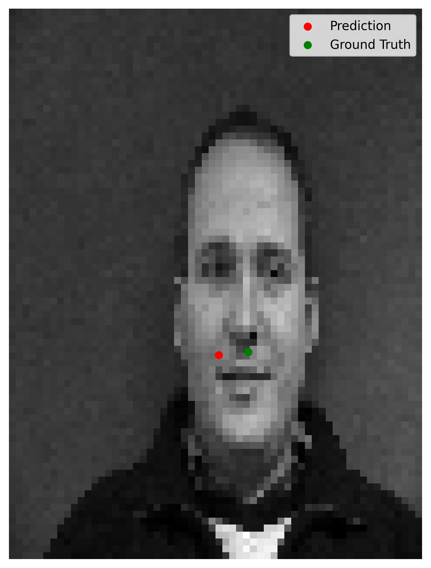
Prediction 2 (inaccurate)
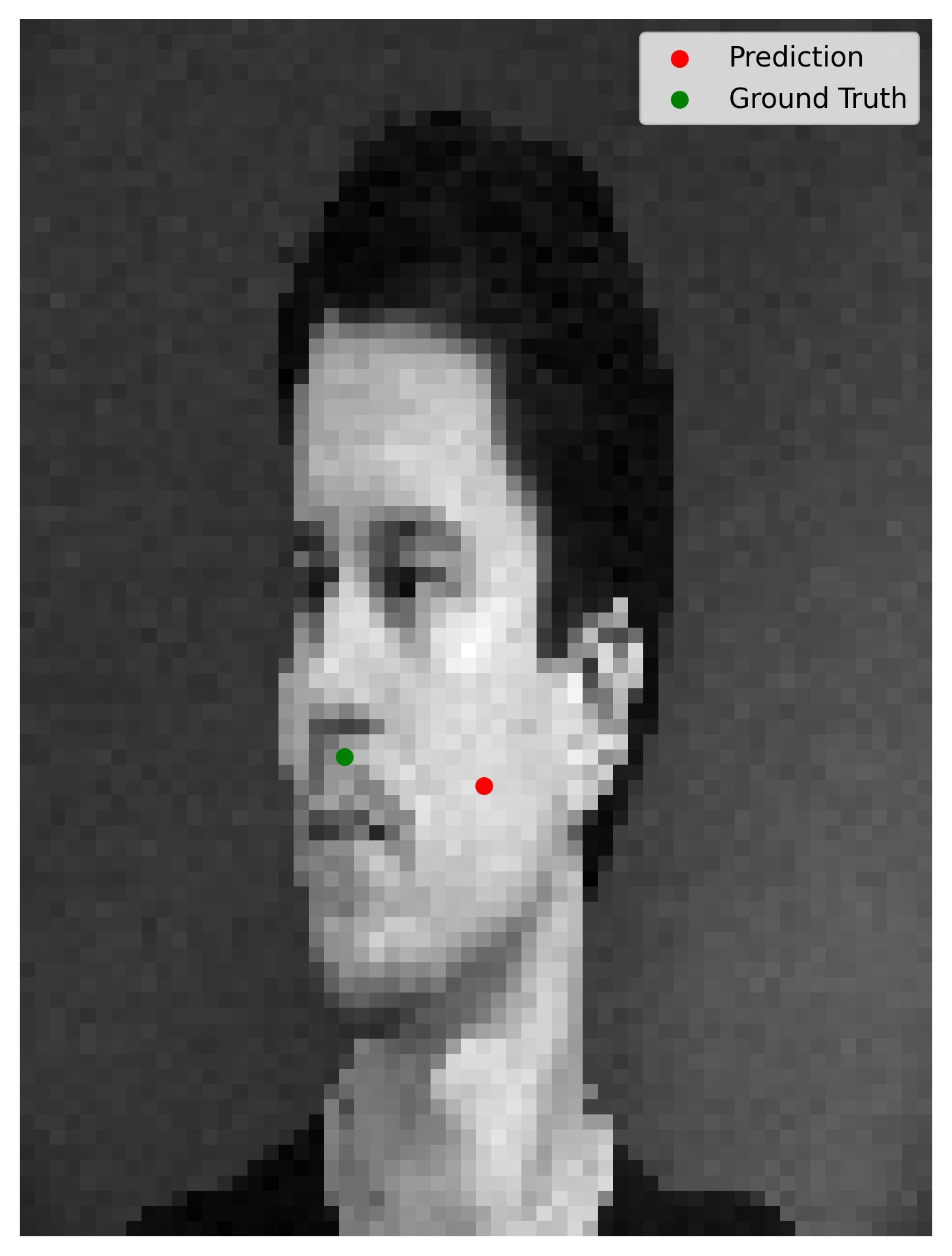
Prediction 3 (inaccurate)
As you can see, the first two images we display acquire pretty satisying predictions. However, the last two has errors in their predictions. Our hyphotesis for the inaccurate predictions is that the model does perform poorly on images where the face isn't straight on the camera and/or in the cases where facial expressions are more pronounced. This is assumed to be due to the limited amount of data and the small size of the model.
Hyperparameter Search
We start our hyperparameter search with exploring learning rates. We test the learning rates displayed on the below plot. No learning rate seems to work better than our initial selection.
Then, we proceed with using a deeper model with 5 convolutional layers that double in the size of the hidden layers for every layer. However, the results also seem to show no credible improvement. The more shallow model is inclided to converge to a "safe" local minima that predicts the average nose tip.
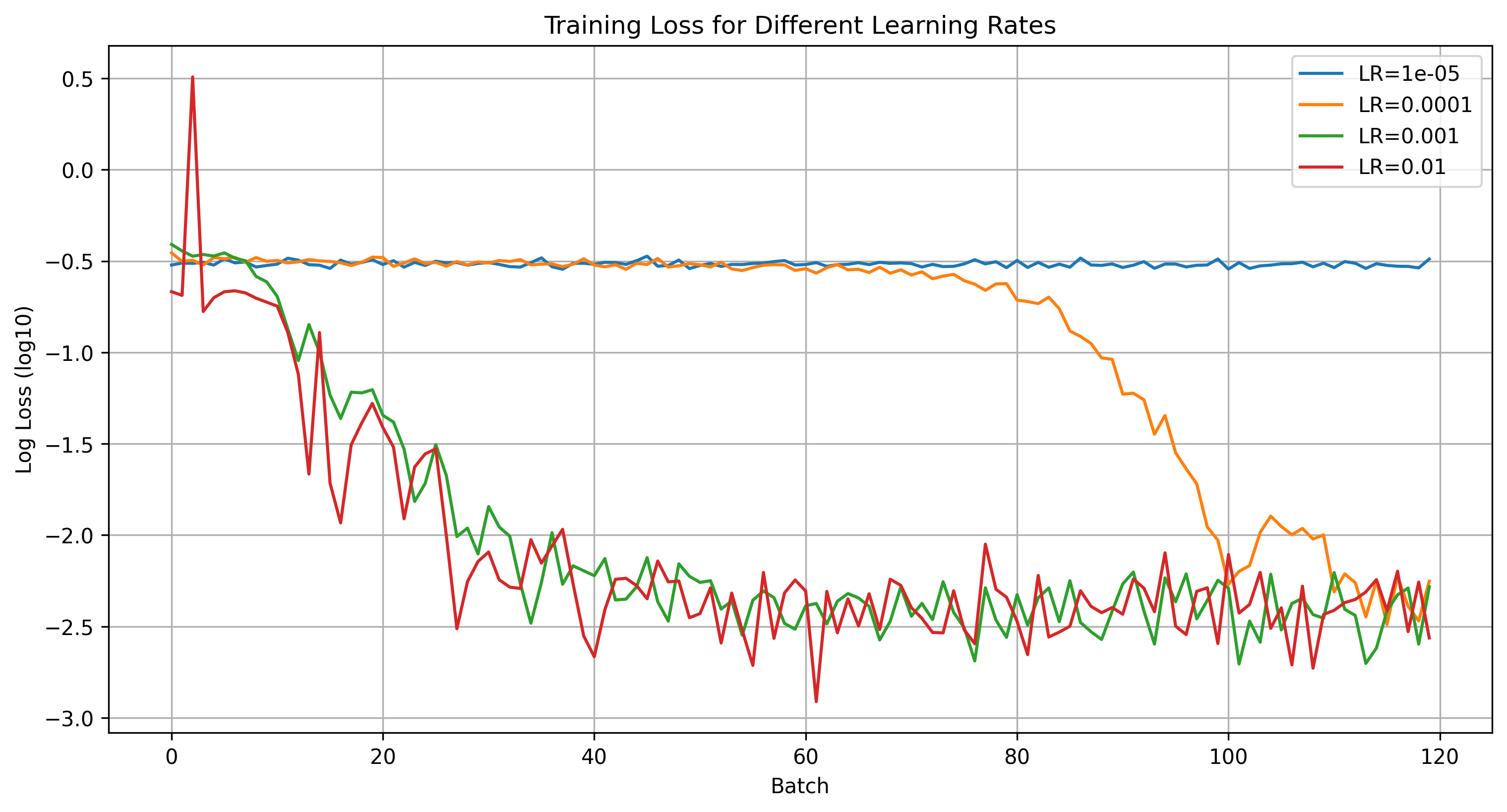
Learning Rate Training Loss Comparison for 3 layer model
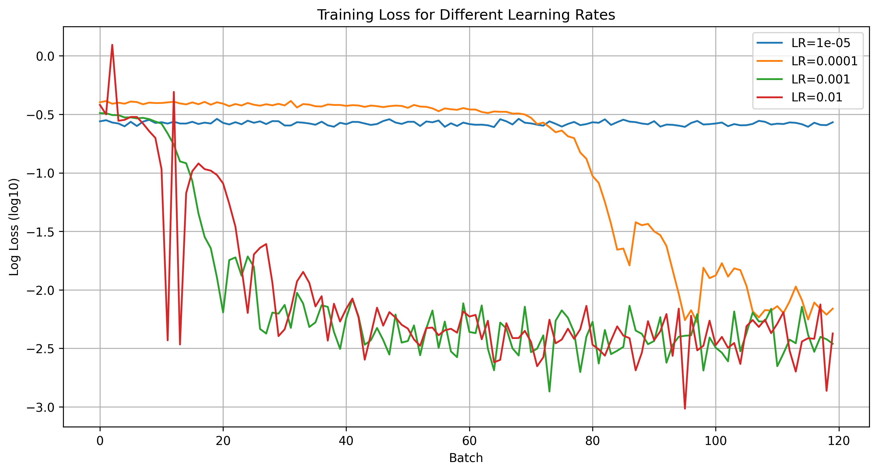
Learning Rate Training Loss Comparison for 5 layer model
Full Facial Keypoint Detection
In this part, we are going to extend the model to detect all the facial keypoints. We are going to run the training procedure on all 58 keypoints that the dataset provides. There are couple changes to the pipeline. To start off, we are going to be having larger input images of size 240x180 as well as data augmentation. Data augmentation is important as we have a small dataset and we don't want to overfit, augmentation enables us to have more data to train on.
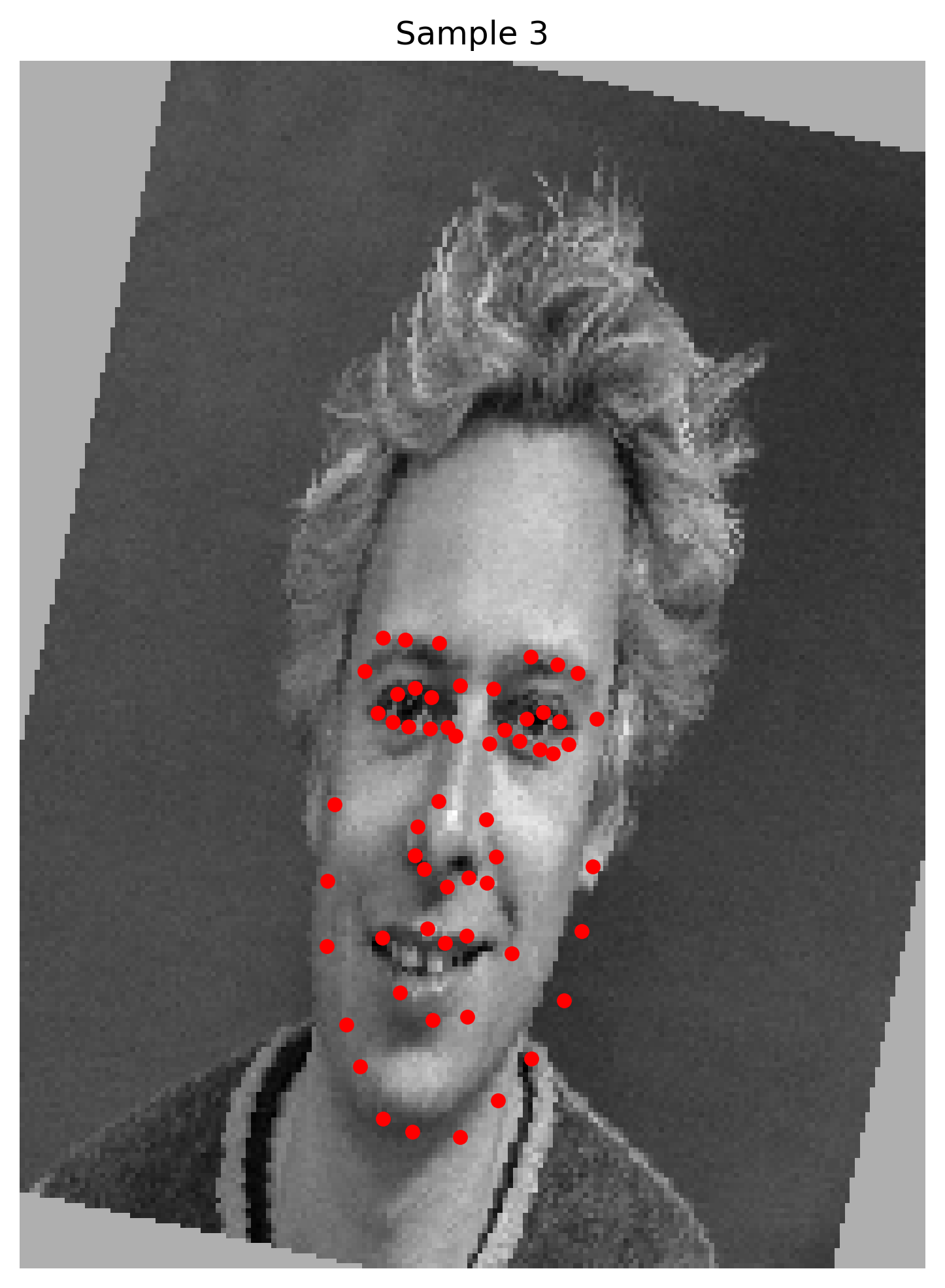
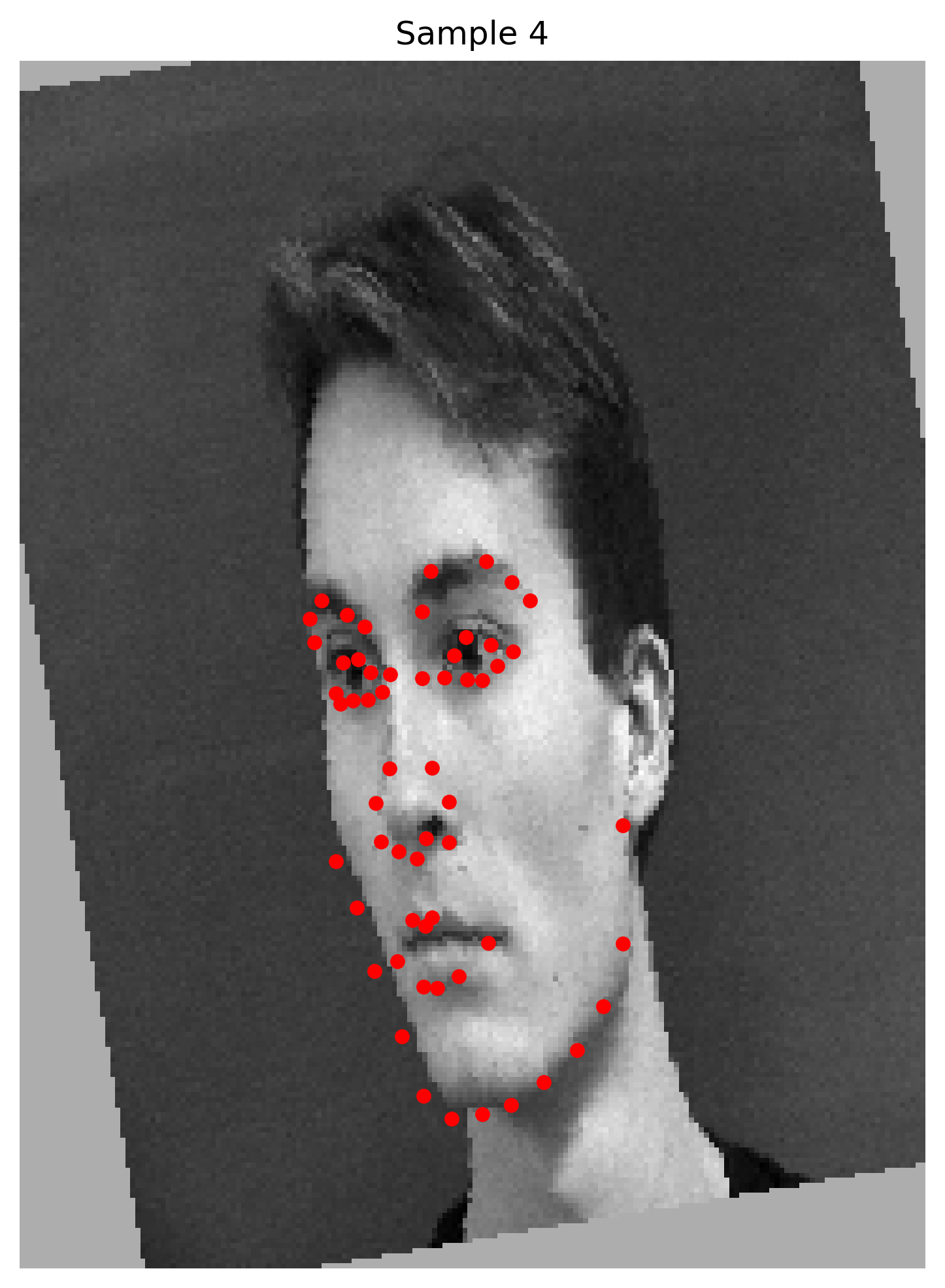
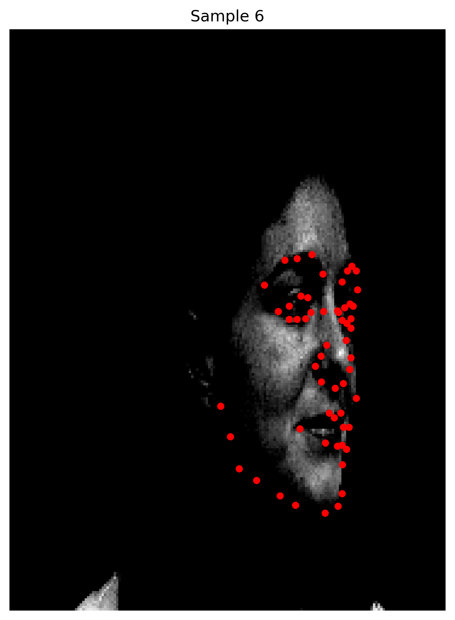
As for the augmentation, we are going to be applying random rotations in range of -15 to 15 degrees, translation in range of -10 to 10 pixels, and color jittering, such as brightness and saturation where we vary the brightness and saturation by +- 25% with probability p=0.3. While doing so, it's important to apply the translational transformation to the keypoints as well. Trying to do so initially caused problems where we weren't able to align the keypoints with the transformed image. Upon investigating, it was found that the rotational matrix that's applied to the keypoints is problematic if the keypoints are not centered around the origin. This was a subtle issue as the computer vision libraries used to rotate the images are based on the assumption of rotating the image from the center. Therefore, we center the keypoints around the origin, apply the rotation, and then shift them back to their original position. For the training, we are going to use a learning rate of 1e-3 as it had worked decently well for the previous task.
Here are some augmented samples from the dataset.
As for the architecture of our model, we are using a 5-layered convolutional model that has 256 channels with two fully conntected layers of 128 and 116 hidden units respectively. The first fully connected layer is followed by a ReLU activation function, and the second layer is followed by a dropout layer with p=0.35 as we noticed that the model shows extreme tendency to overfit, most probably due to the small amount of data we have.
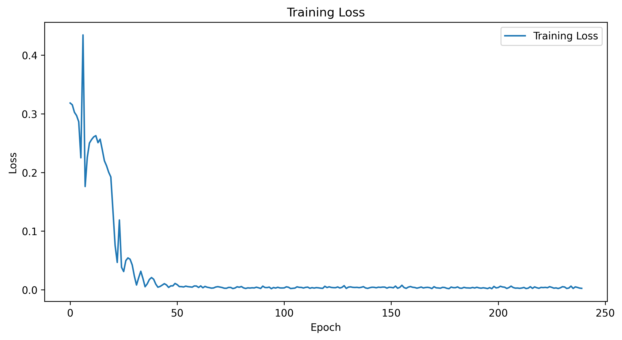
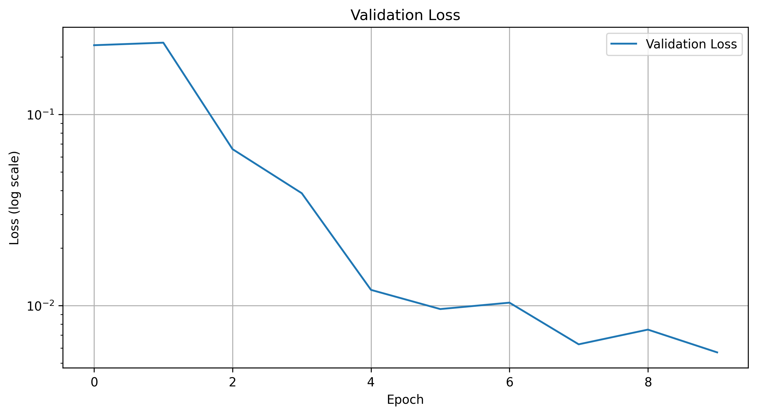
Here are the progression of the training and validation losses for the model.
Training Loss
Validation Loss
Here are the visualizations of the filters every other layer throughout the model
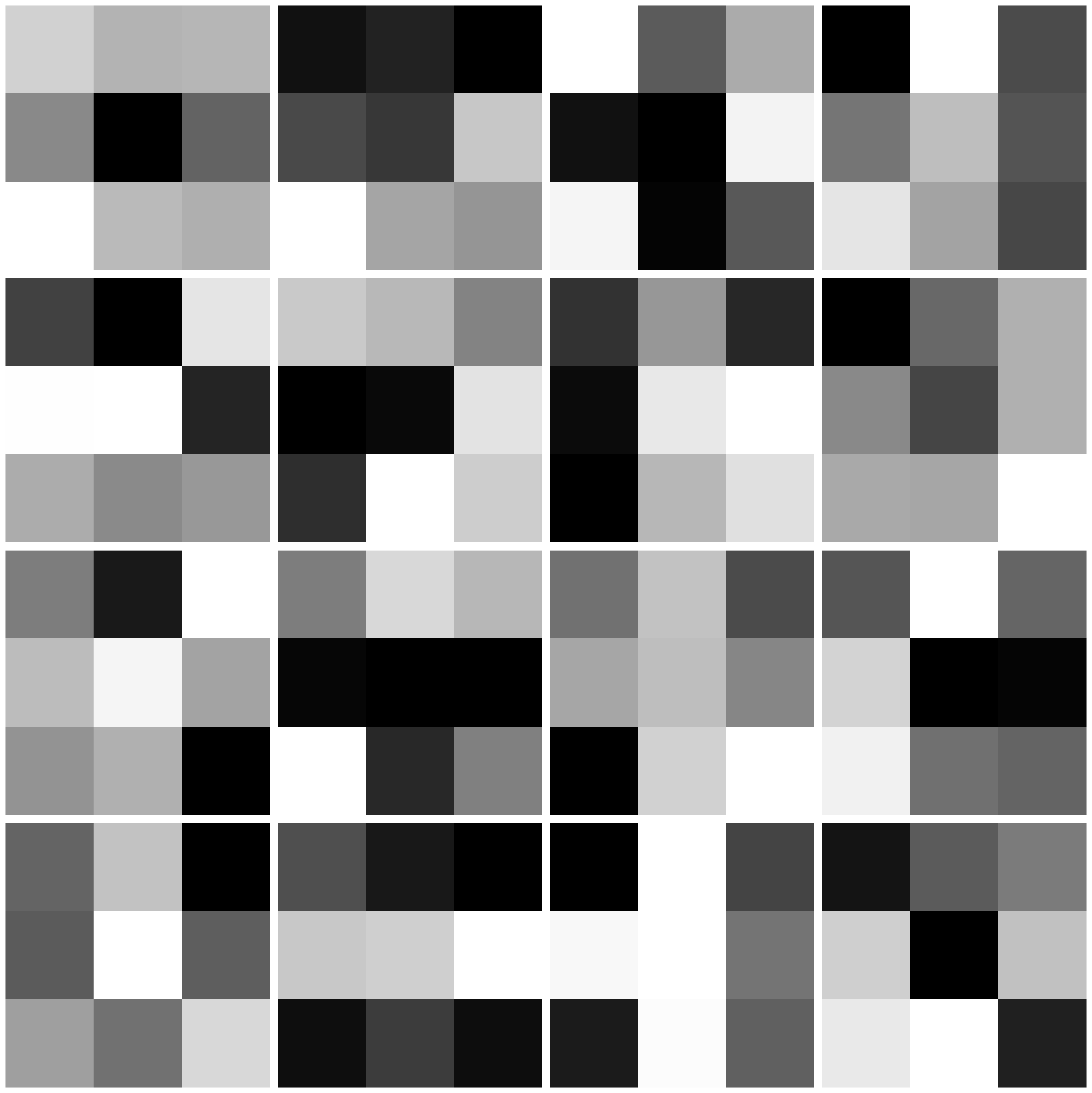
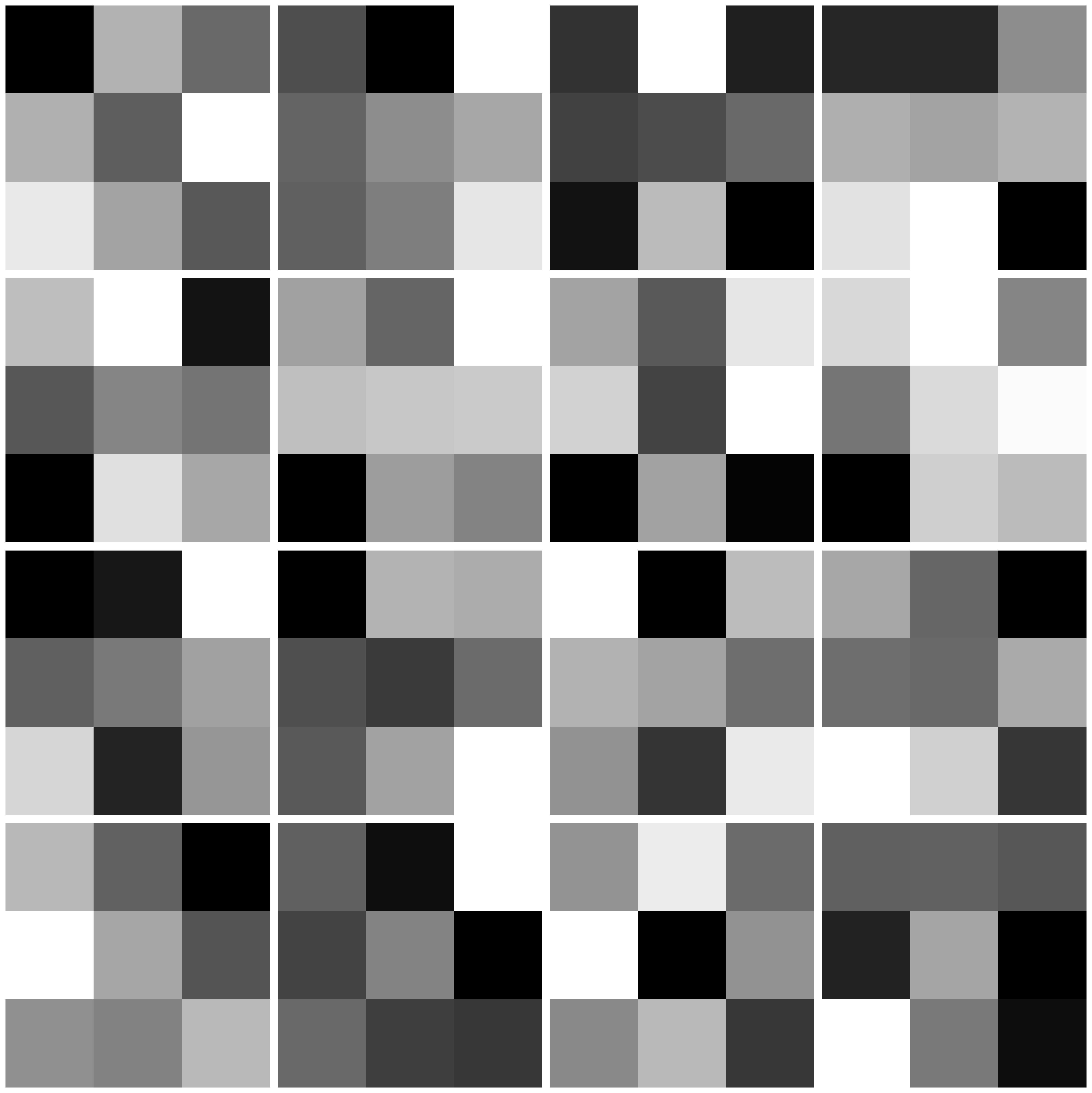
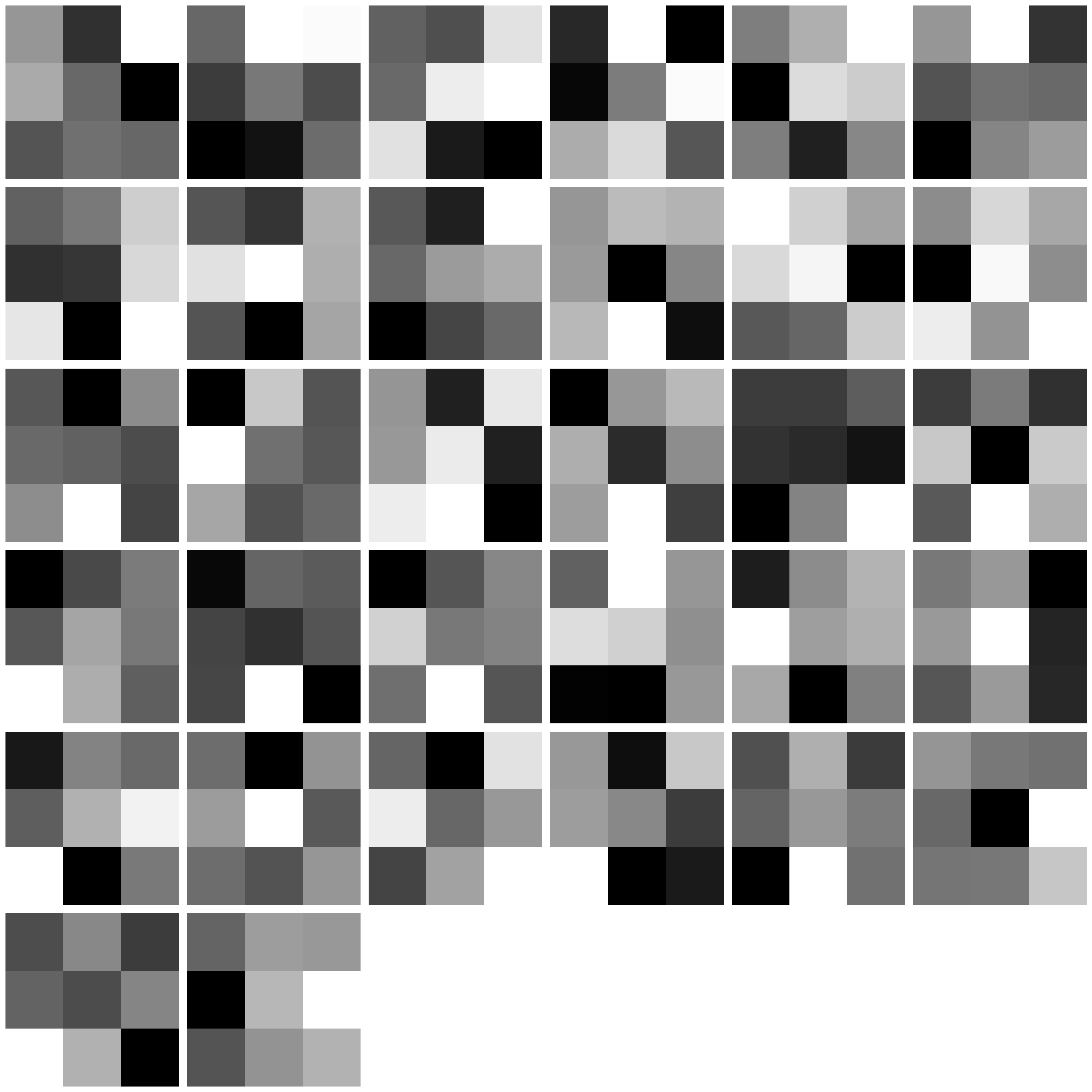
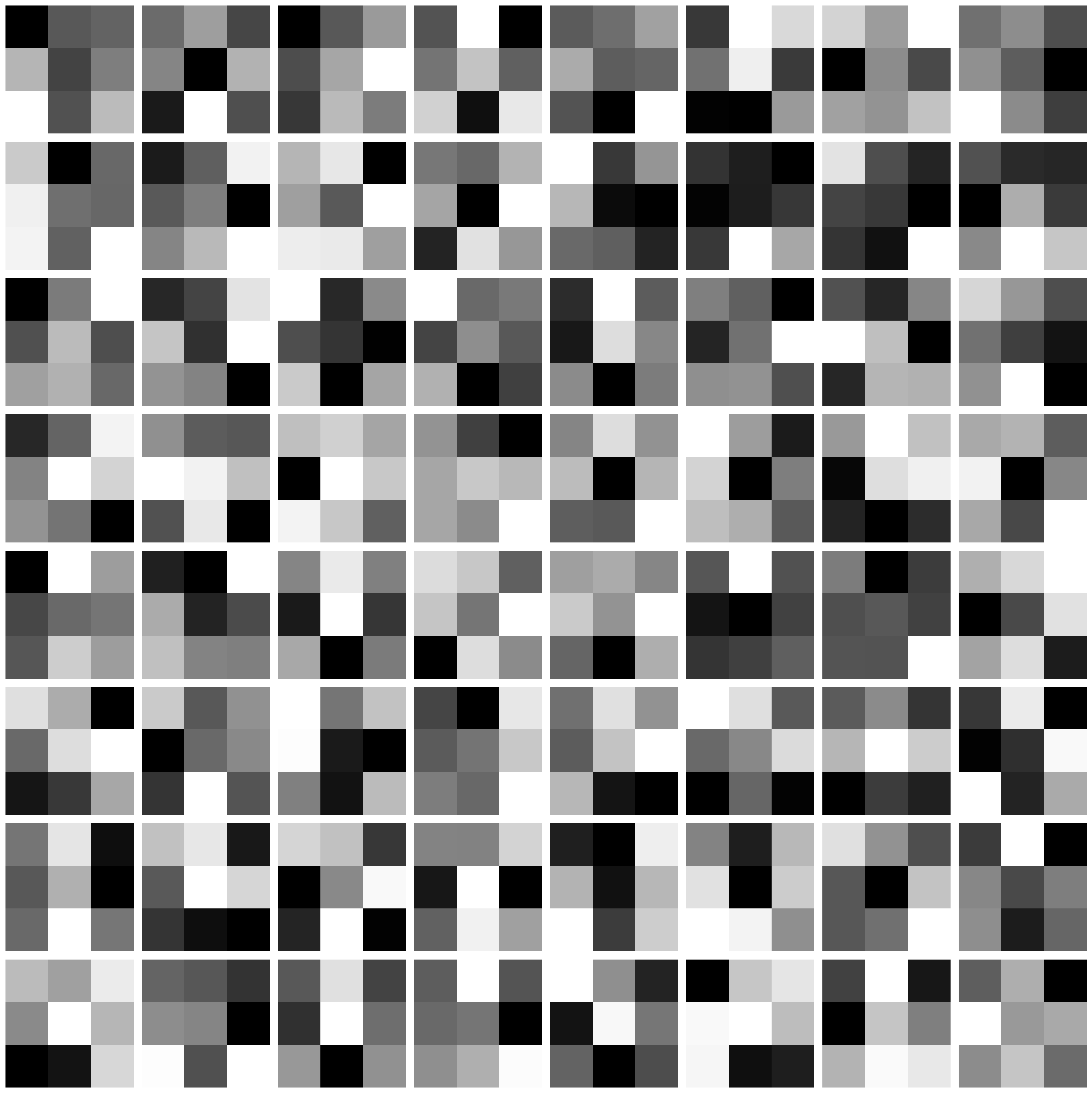
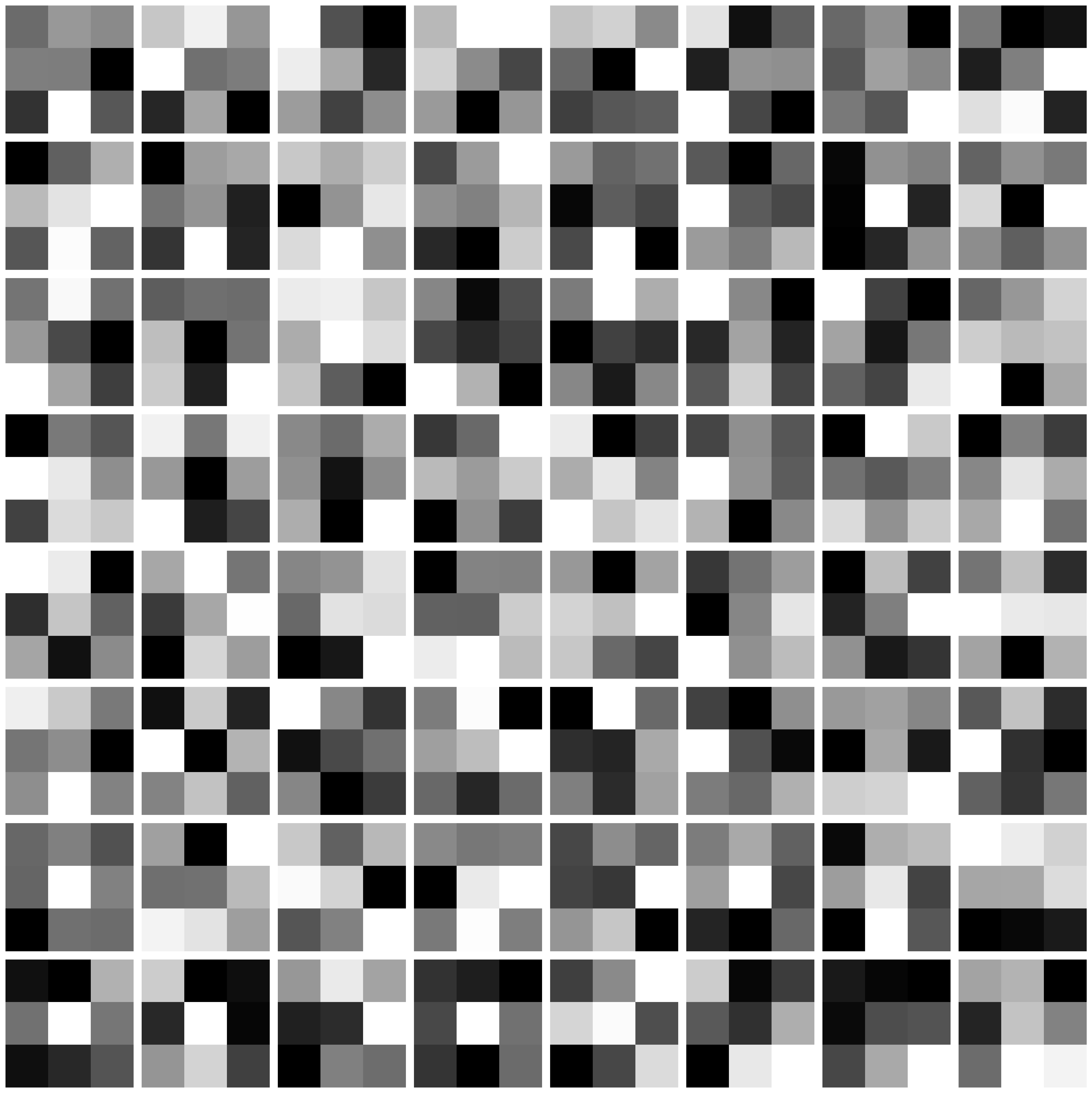
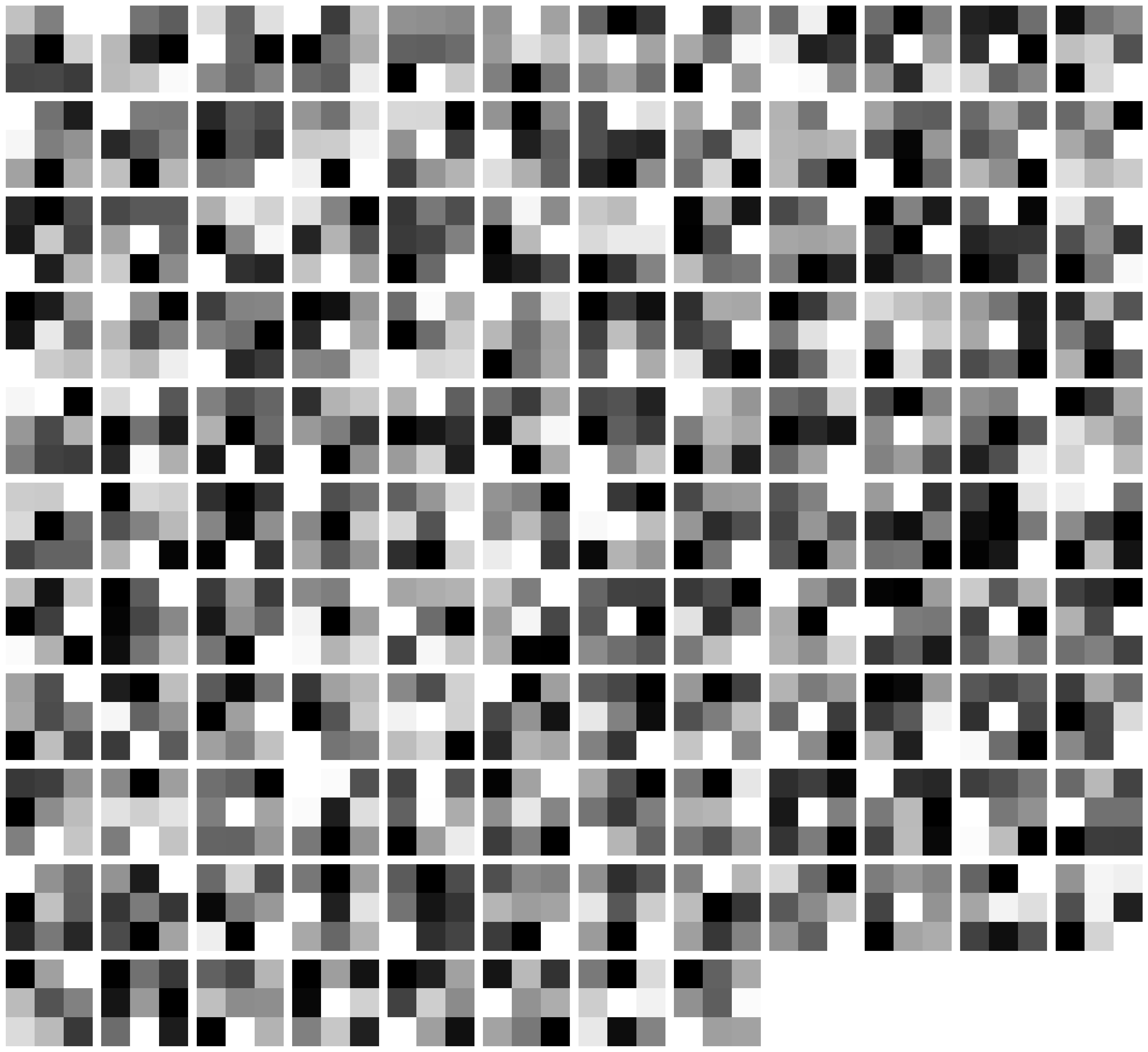
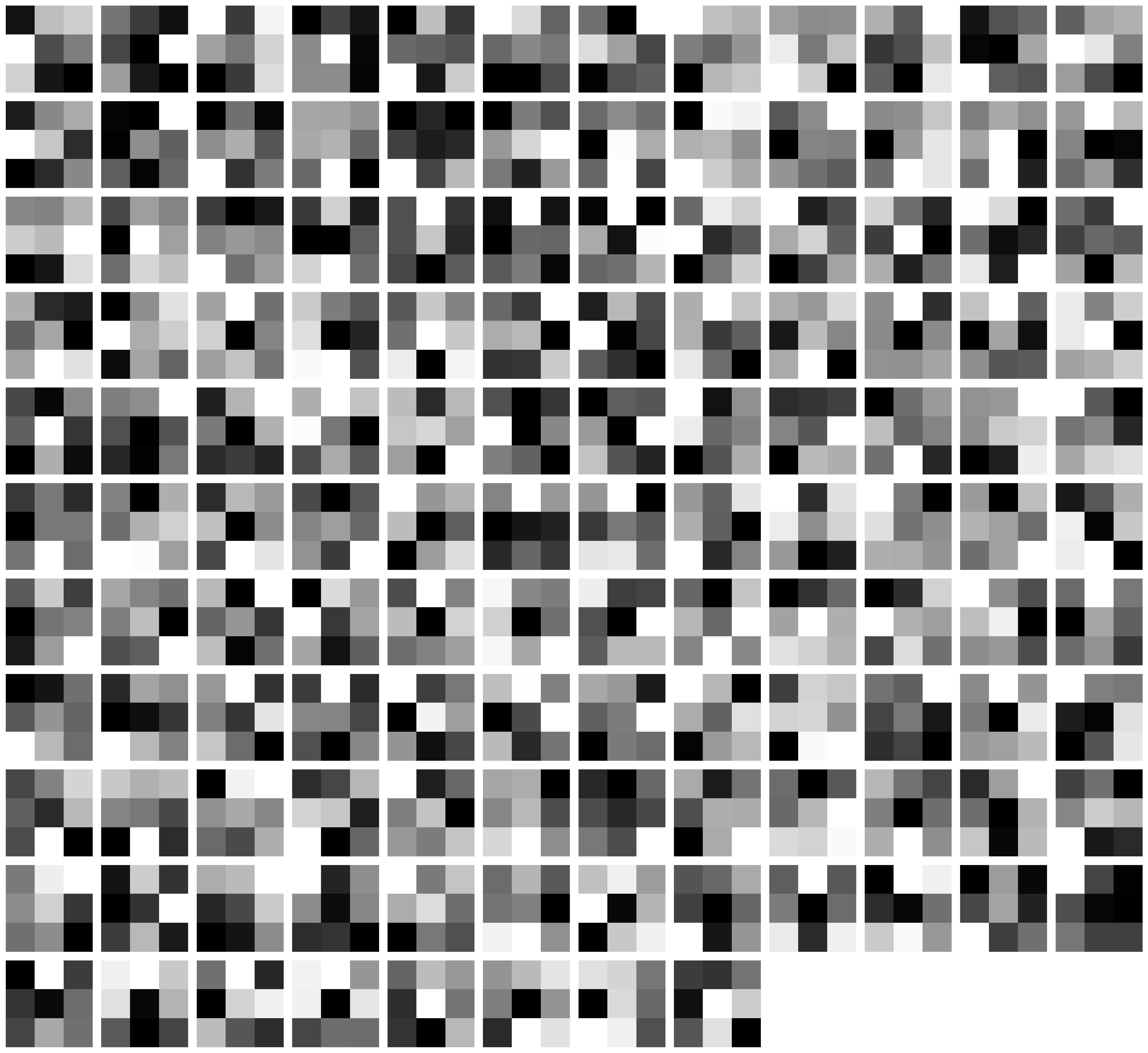
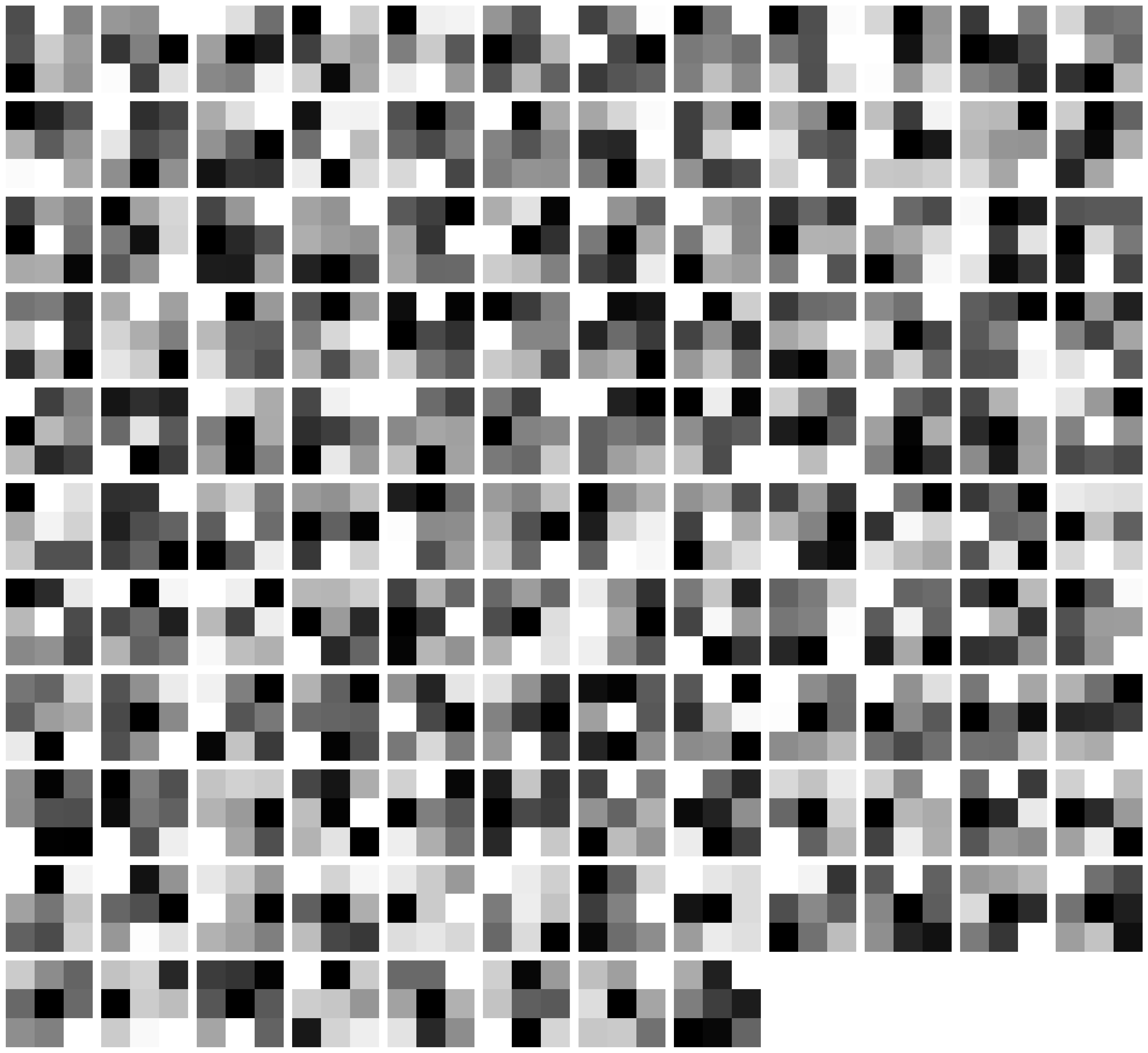
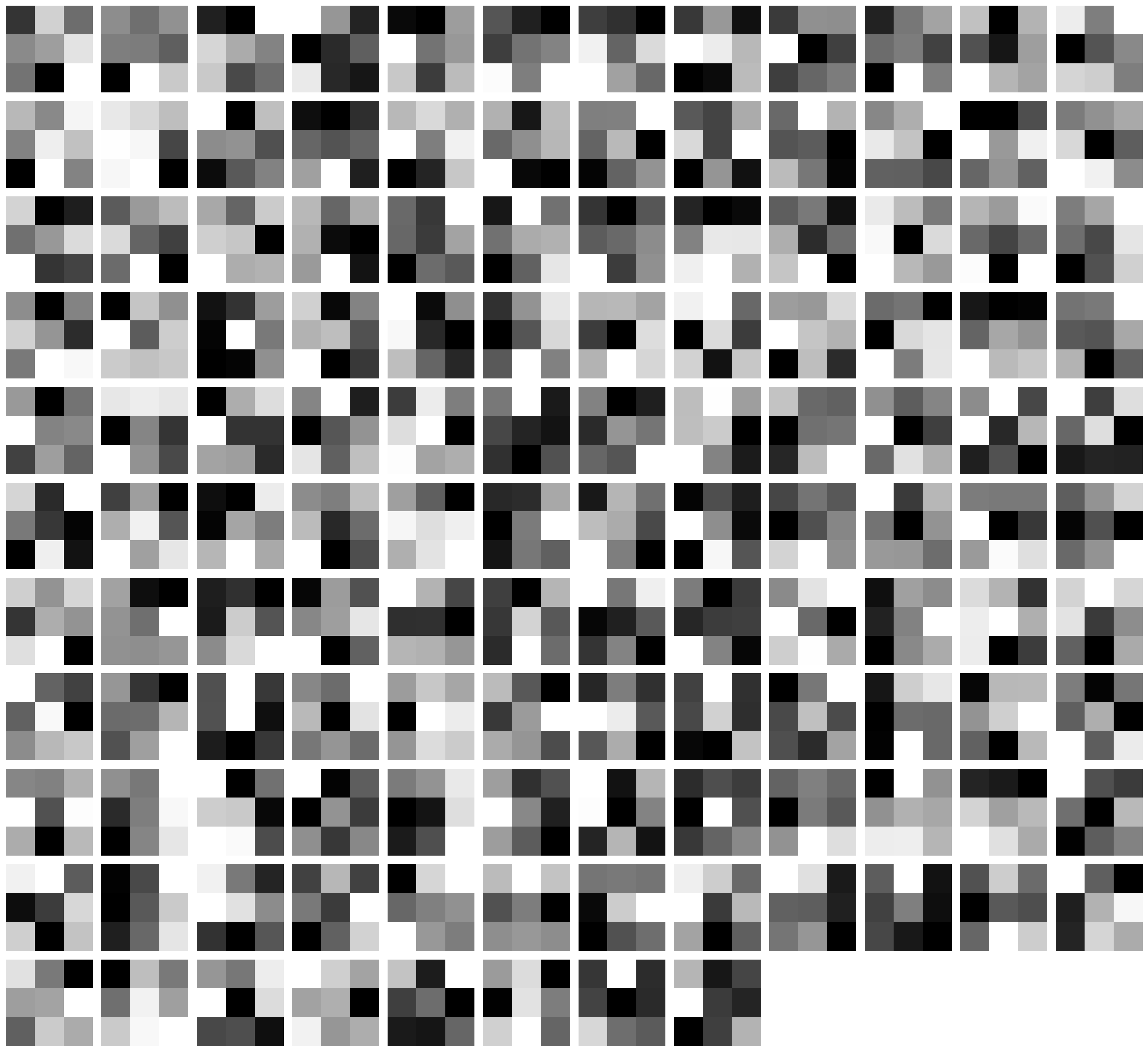
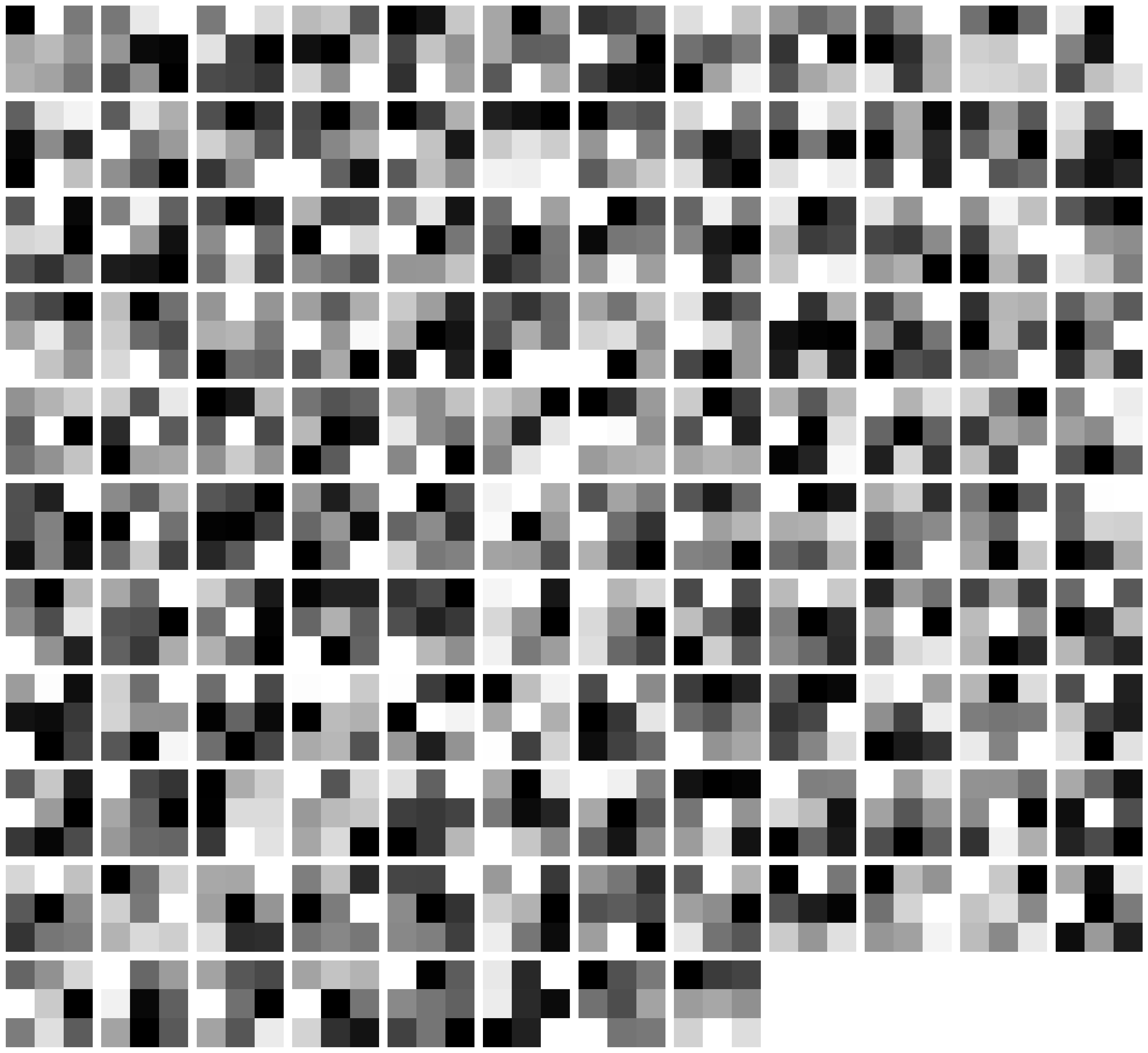
As you can see, we tend to have couple unused (dead) filters throughout our model. This is probably due to the lack of data and the overcomplexity of the model because the model doesn't need to activate all the filters to get a good prediction.
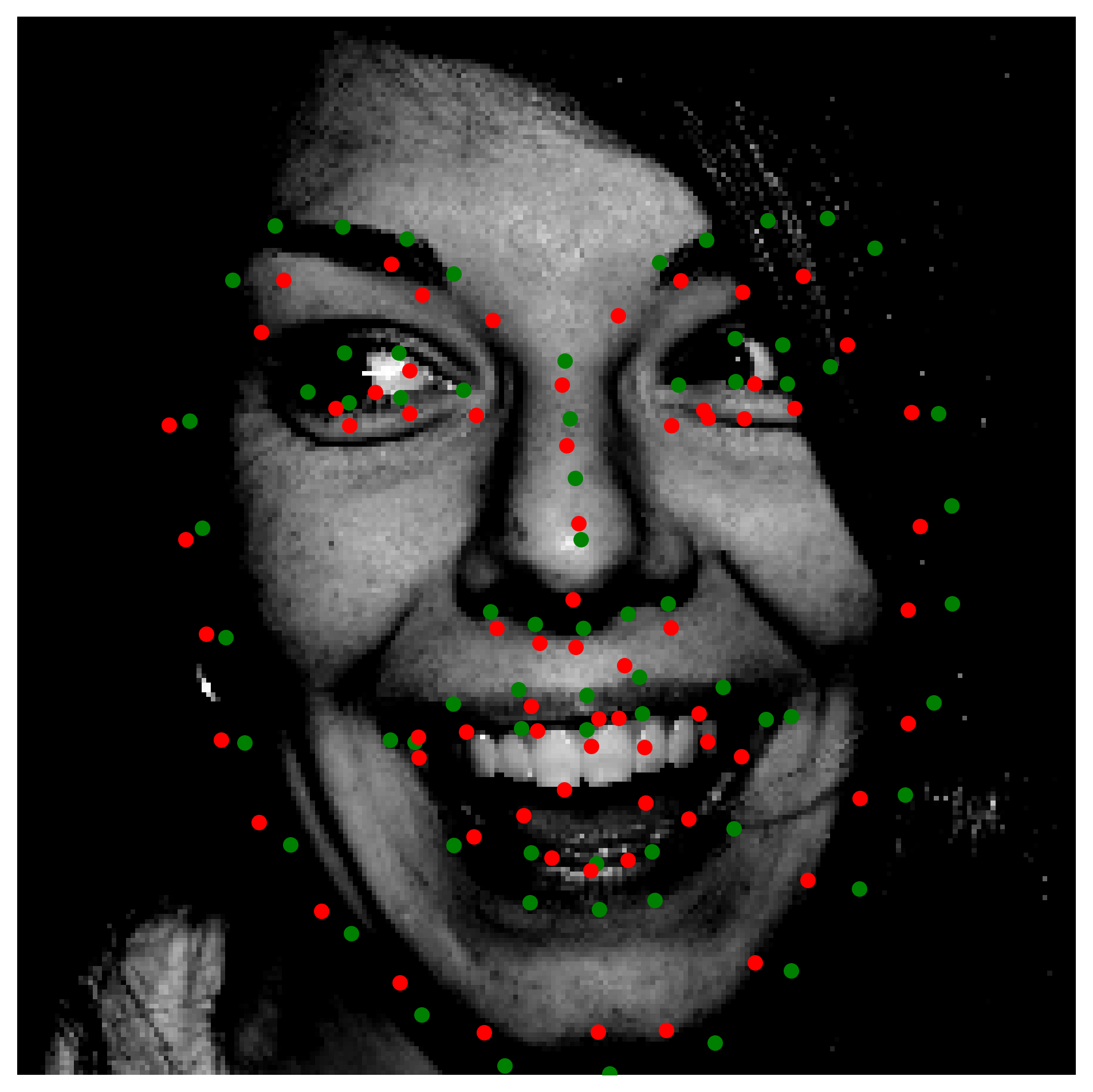
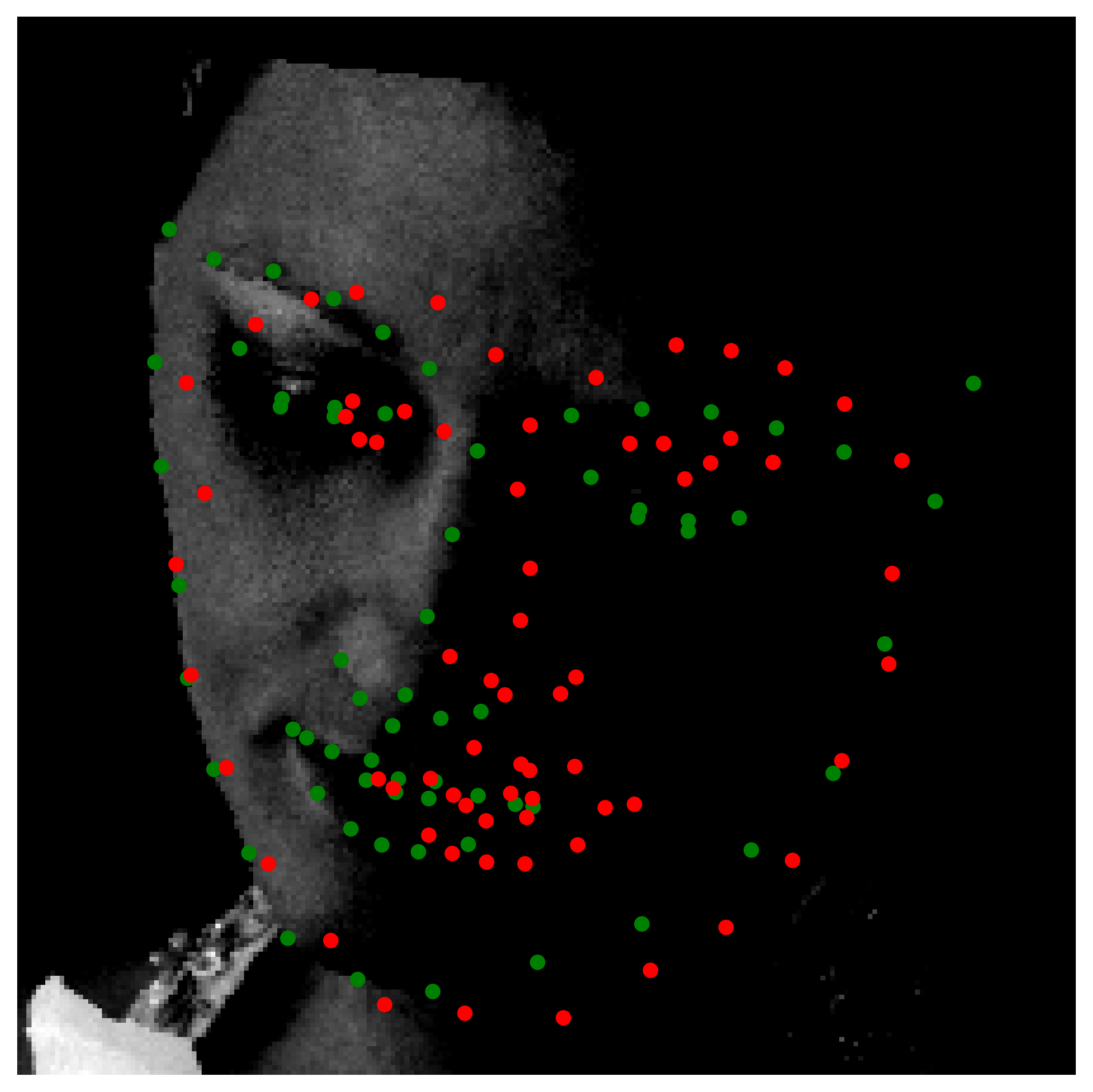
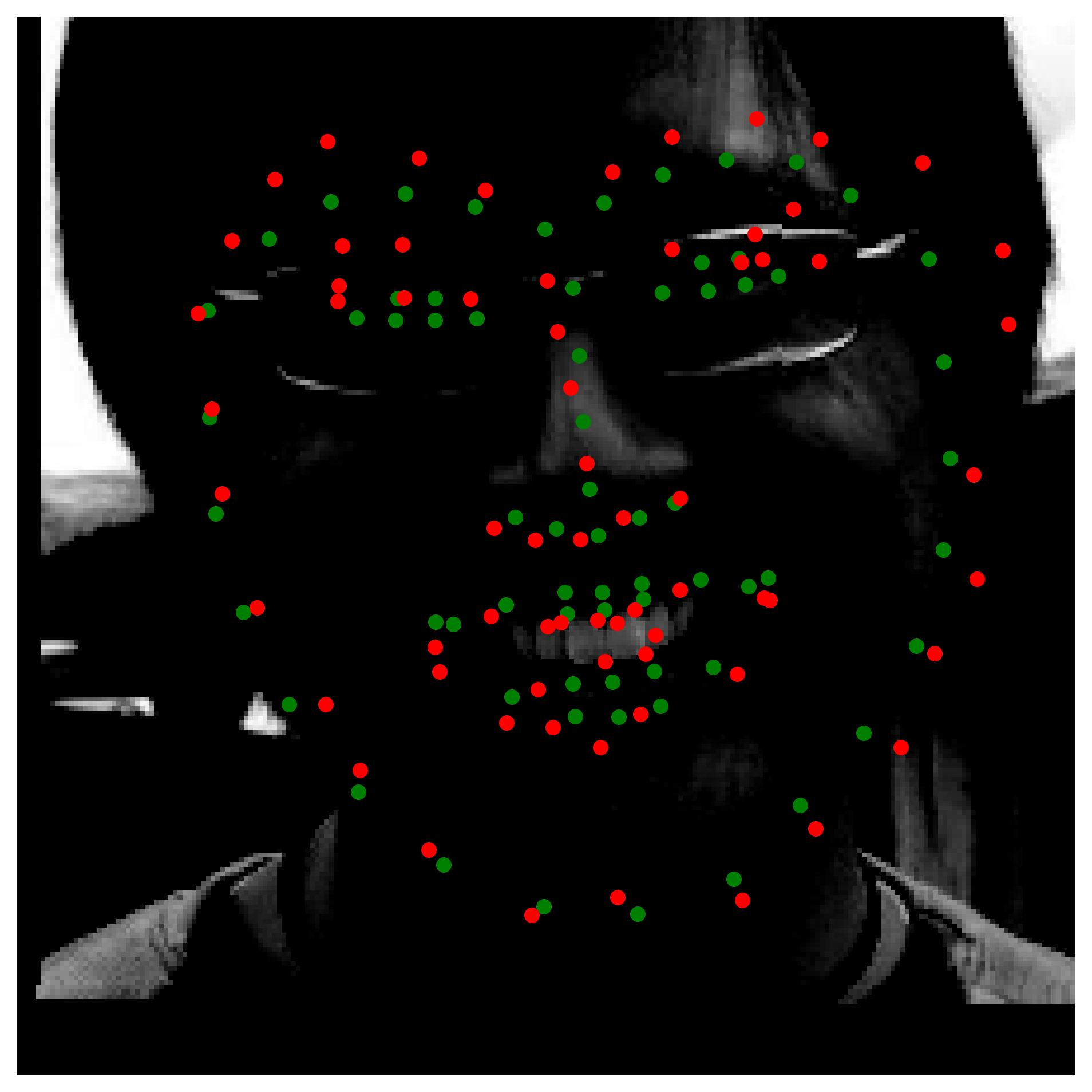
Here are some predictions

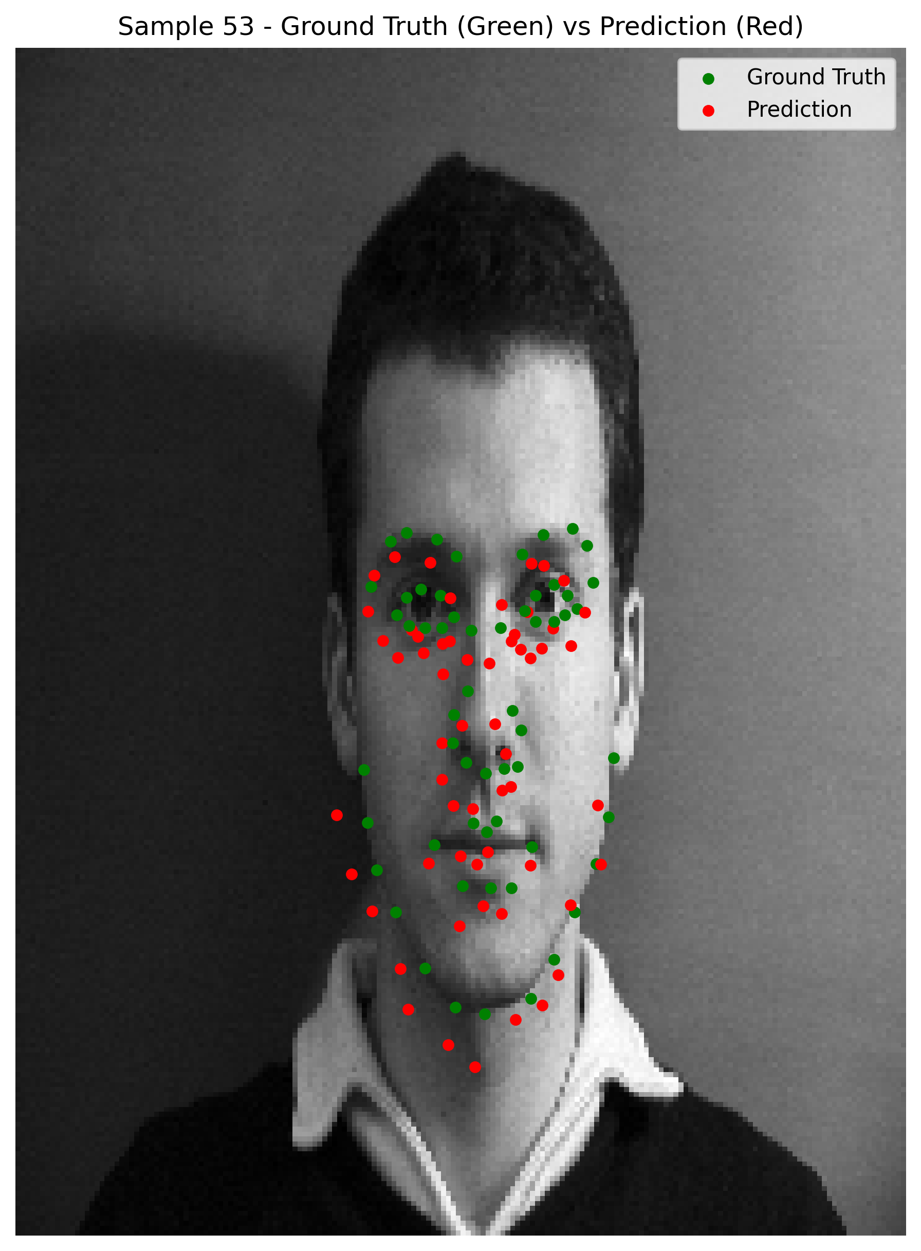
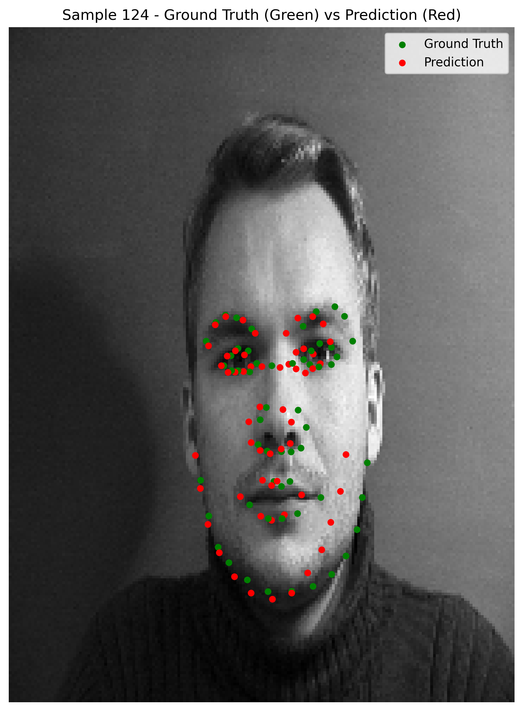
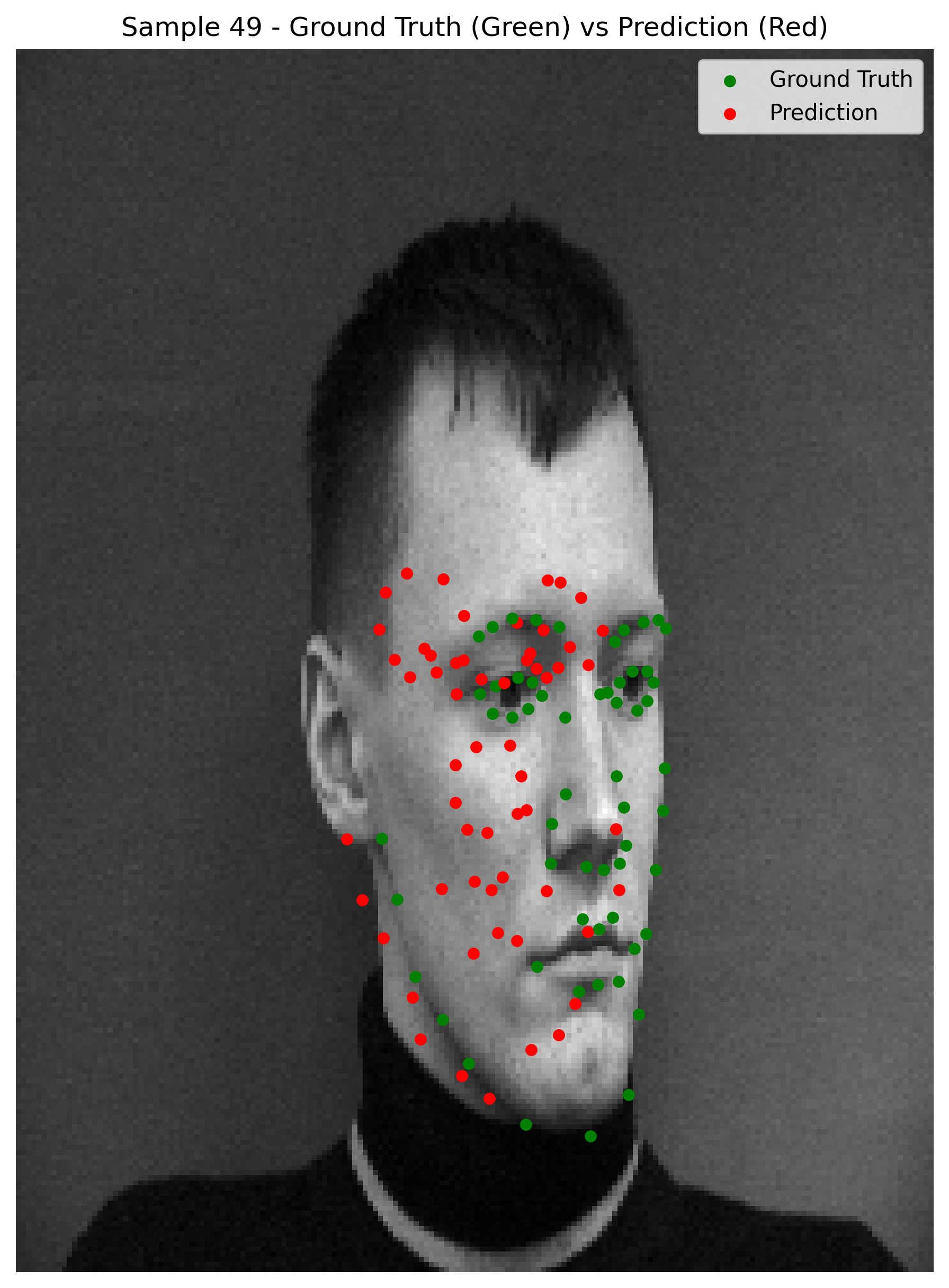
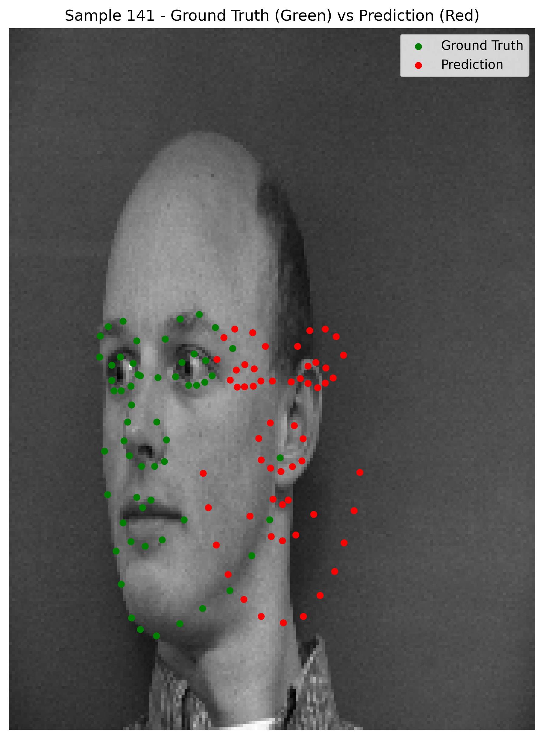
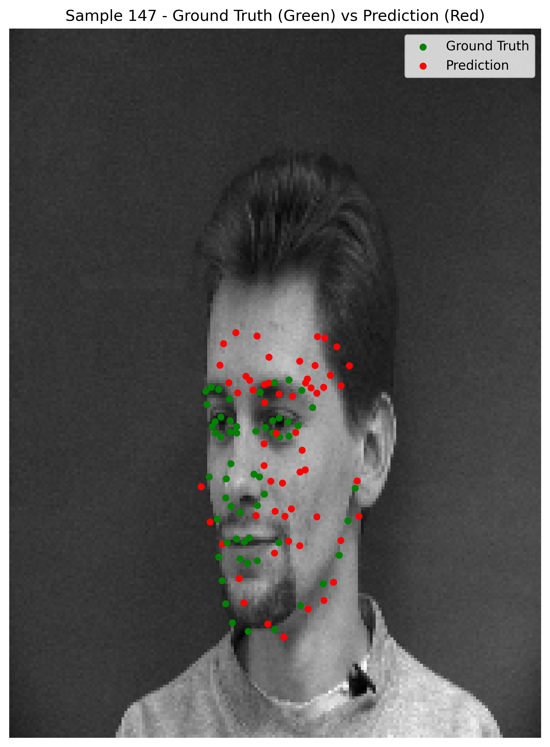
When observing the results, we can see that the model does relatively well on cases where the face is straight on the camera and the facial expressions are not too pronounced. However, the the model seems to be predicting the average keypoints when the face is rotated.
Increasing the Model Size
In this part, we are going to increase the model size as well as using a quite larger dataset to see if we can improve the model's performance. As for our model, we are going to use a ResNet18 model with 18 layers, with minor changes to the initial convolution layer, to accmodate our grayscale images as well as adapting the output layer to match the number of keypoints. We are going to use the Adam optimizer with a learning rate of 1e-3. We are going to use the same data augmentation techniques as in the previous part. After training with the initial setup, unsatisfied with the results, we have implemented a learning rate scheduler with gamma 0.1 and step size 5.
One other modification that we did was to the loss function we used. Instead of using MSE as we did for the previous parts, we have decided to use cross-entropy loss instead as we didn't get satisfactory results from the MSE training approaches. We believe cross-entropy loss was a better choice than MSE for the task of predicting heatmaps because it treats the heatmaps as probability distributions rather than just pixel-wise intensity values. In landmark detection, the goal is to predict heatmaps where the pixel values encode the likelihood of a landmark’s position. Cross-entropy loss penalizes the difference between the predicted probability distribution and the ground-truth Gaussian heatmap more effectively by focusing on reducing errors where the target probabilities are high (e.g., near the landmark peak). In contrast, MSE equally penalizes all pixel-wise differences, including areas far from the landmark where values are already near zero, which can lead to slower convergence and less precise localization. Cross-entropy encourages sharper, peaked predictions and helps the model concentrate on accurately estimating the spatial distribution of landmarks, improving overall precision and robustness in landmark localization.
The last modification that was made was to increase the size of the bounding box the dataset offers by 1.2, as the bounding box wasn't manually generated and the algorithm used to generate was commonly cropping parts of the face. Before proceeding to the loss progression and predictions, let's observe some samples from our dataloader after augmentation.
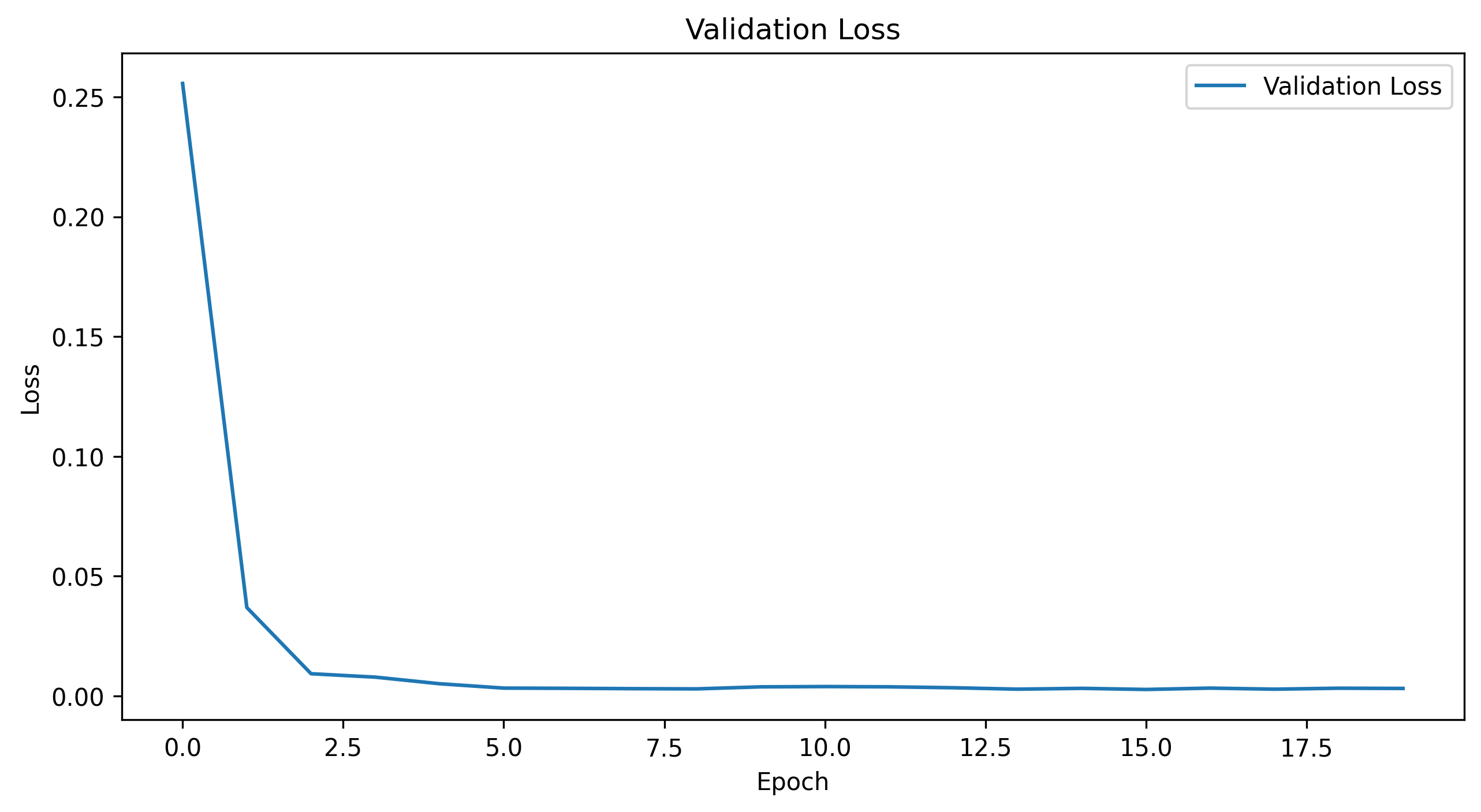
Loss Progression
Training Loss for 10 Epochs
Validation Loss for 10 Epochs
Training Loss for 16 Epochs
Validation Loss for 16 Epochs
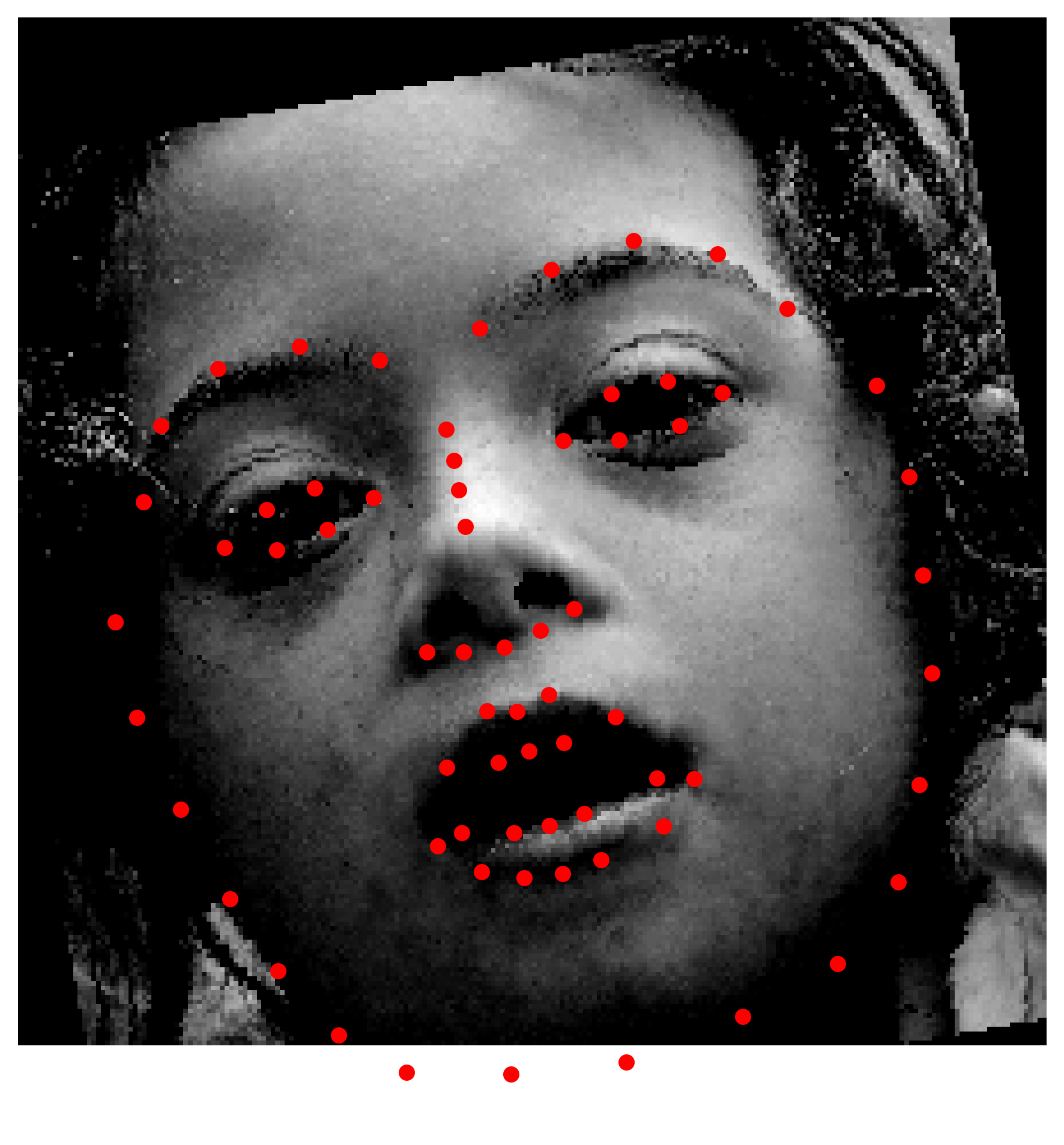
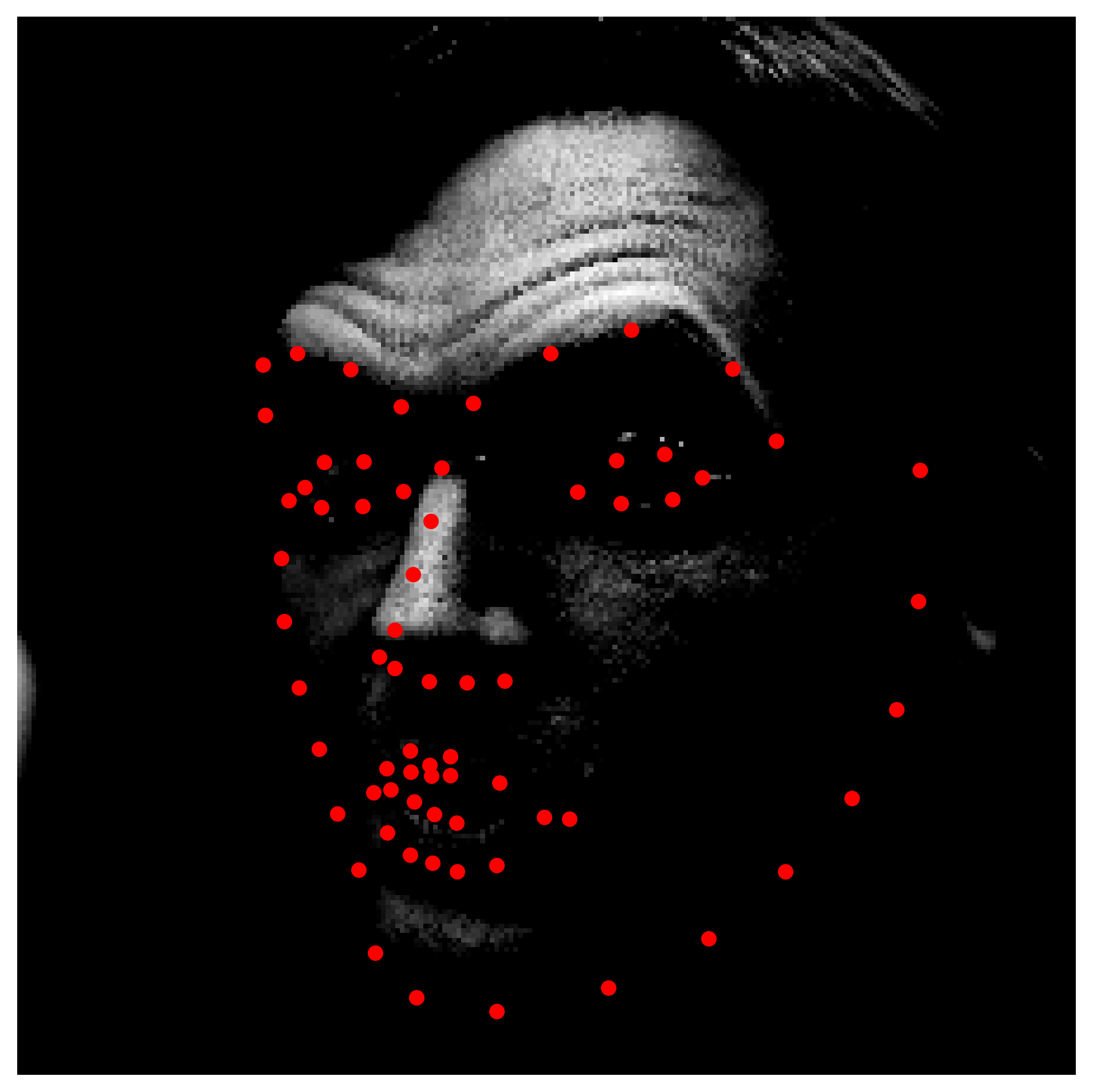
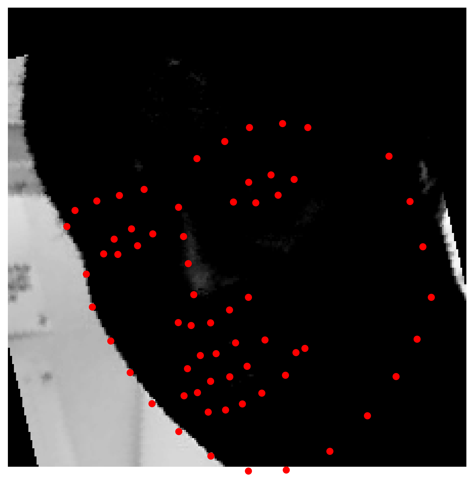
10 Epochs Predictions
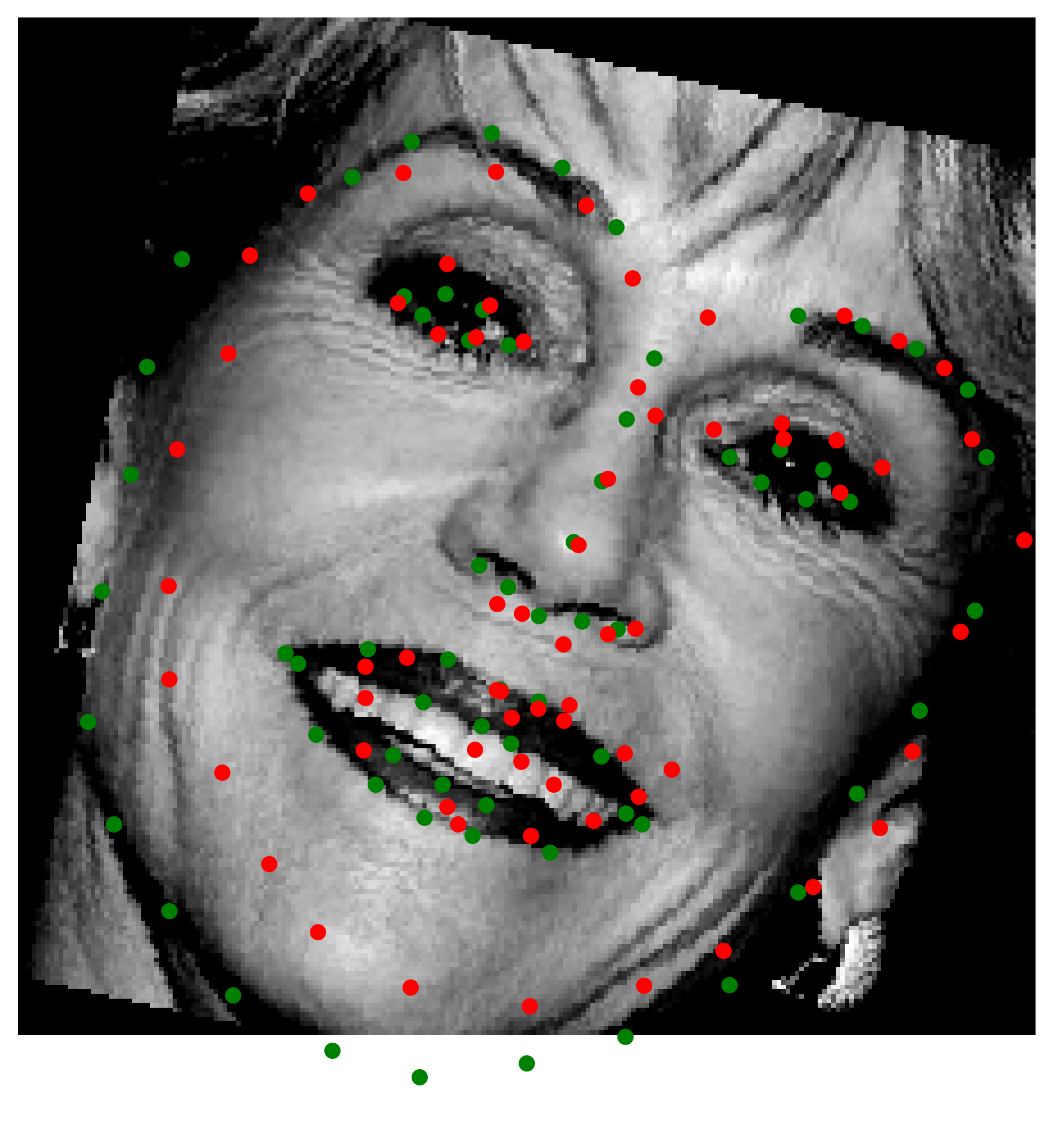
16 Epochs Predictions
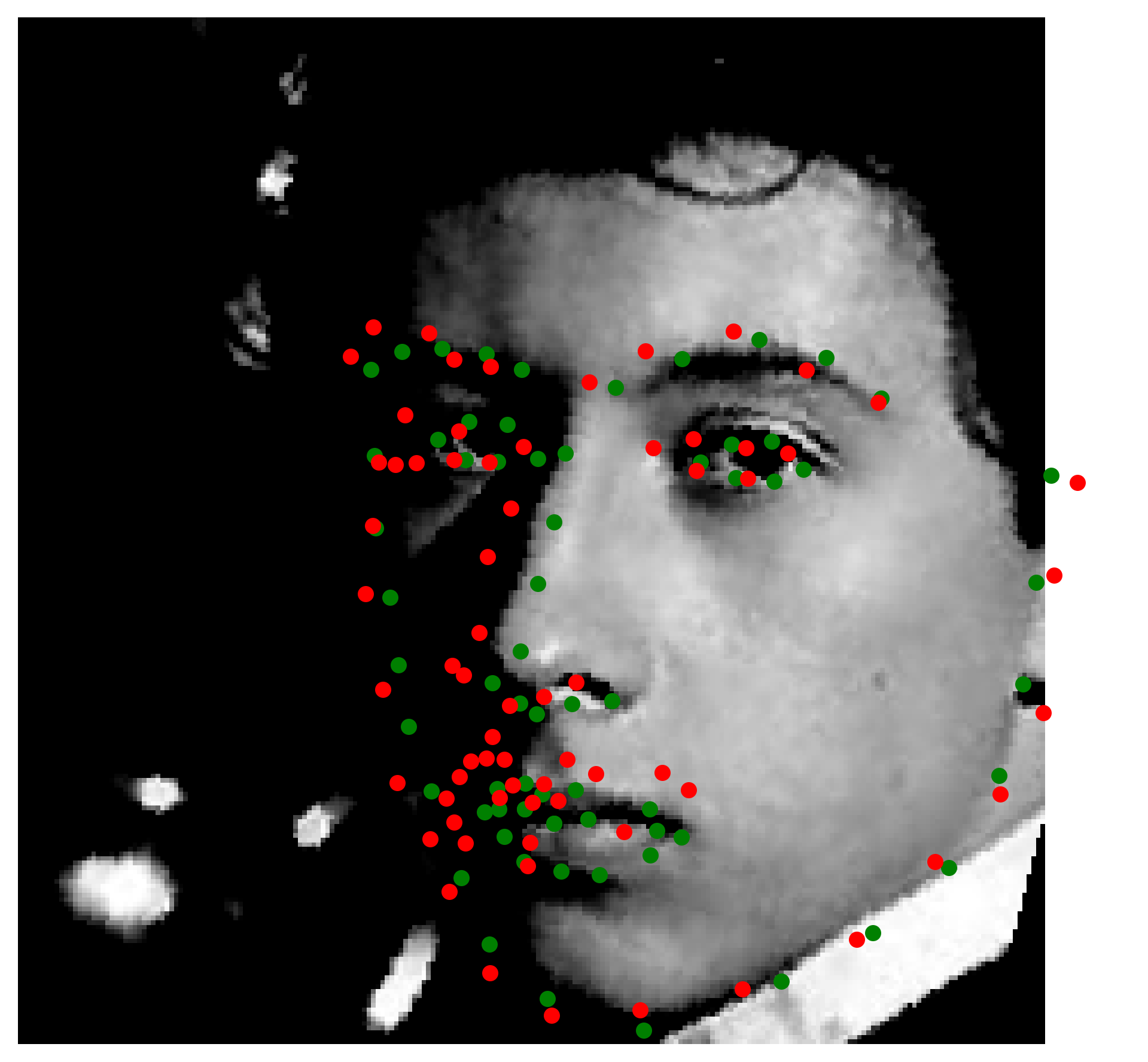
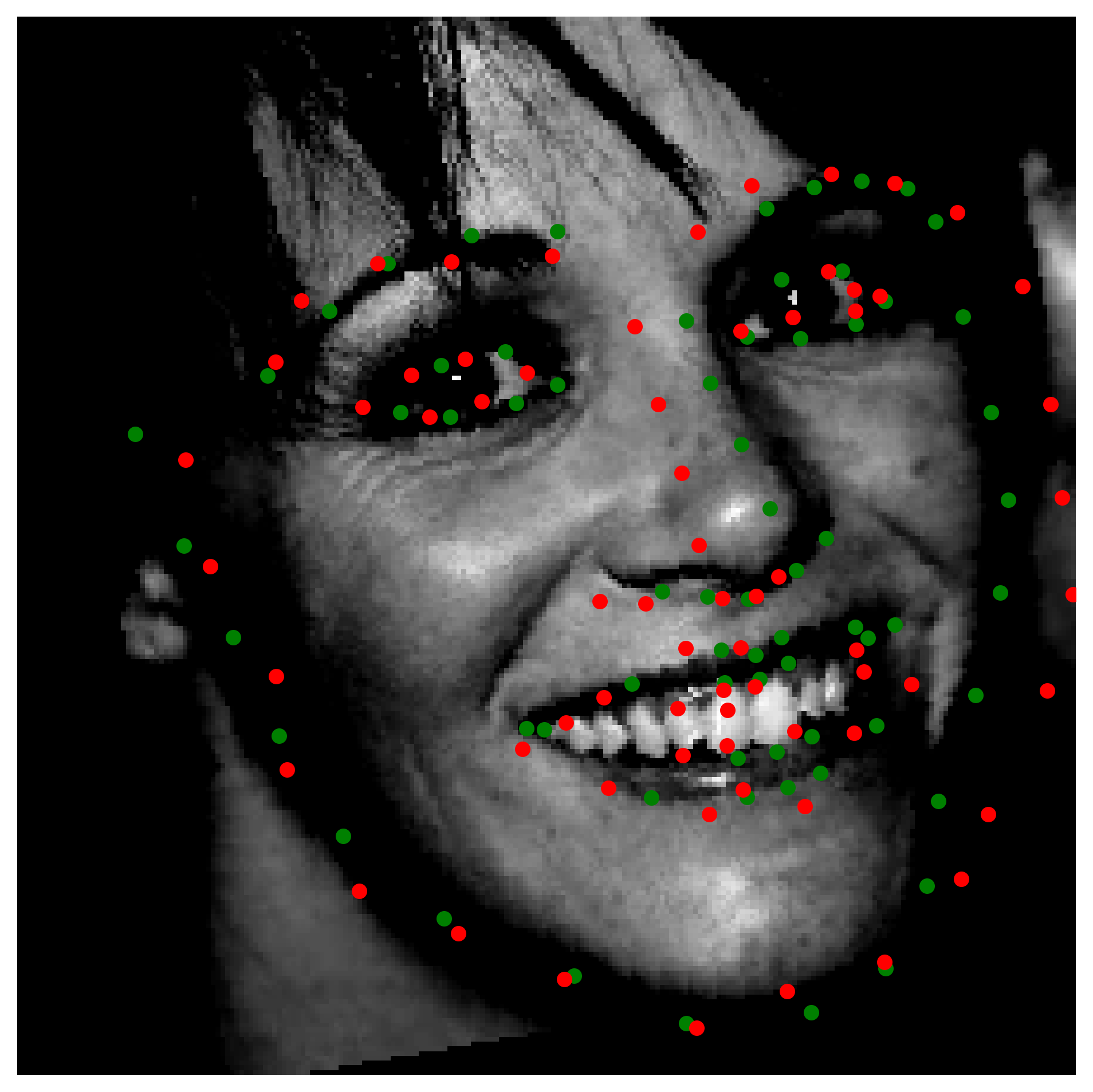
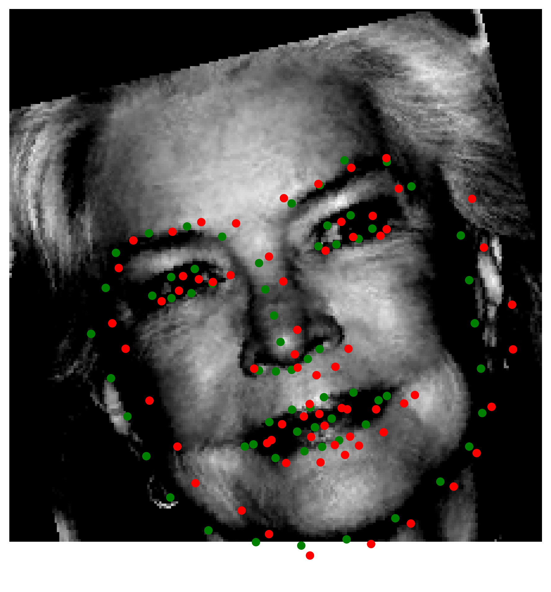
Observing the predictions, it's safe to say that our model does quite a better job than the previos one that was trained on a limited dataset. Most of the results along the quality of the better predictions displayed. A common pattern we noticed for the inaccurate predictions is that they tend to share a 3 degrees of freedom on the orientation of the face. That is, for the faces where there is rotation on the y axis as well as the z axis, the model tends to get inaccurate. This could be explained by the fact that we can't augment the data to include such rotations if the data is limited for such examples.
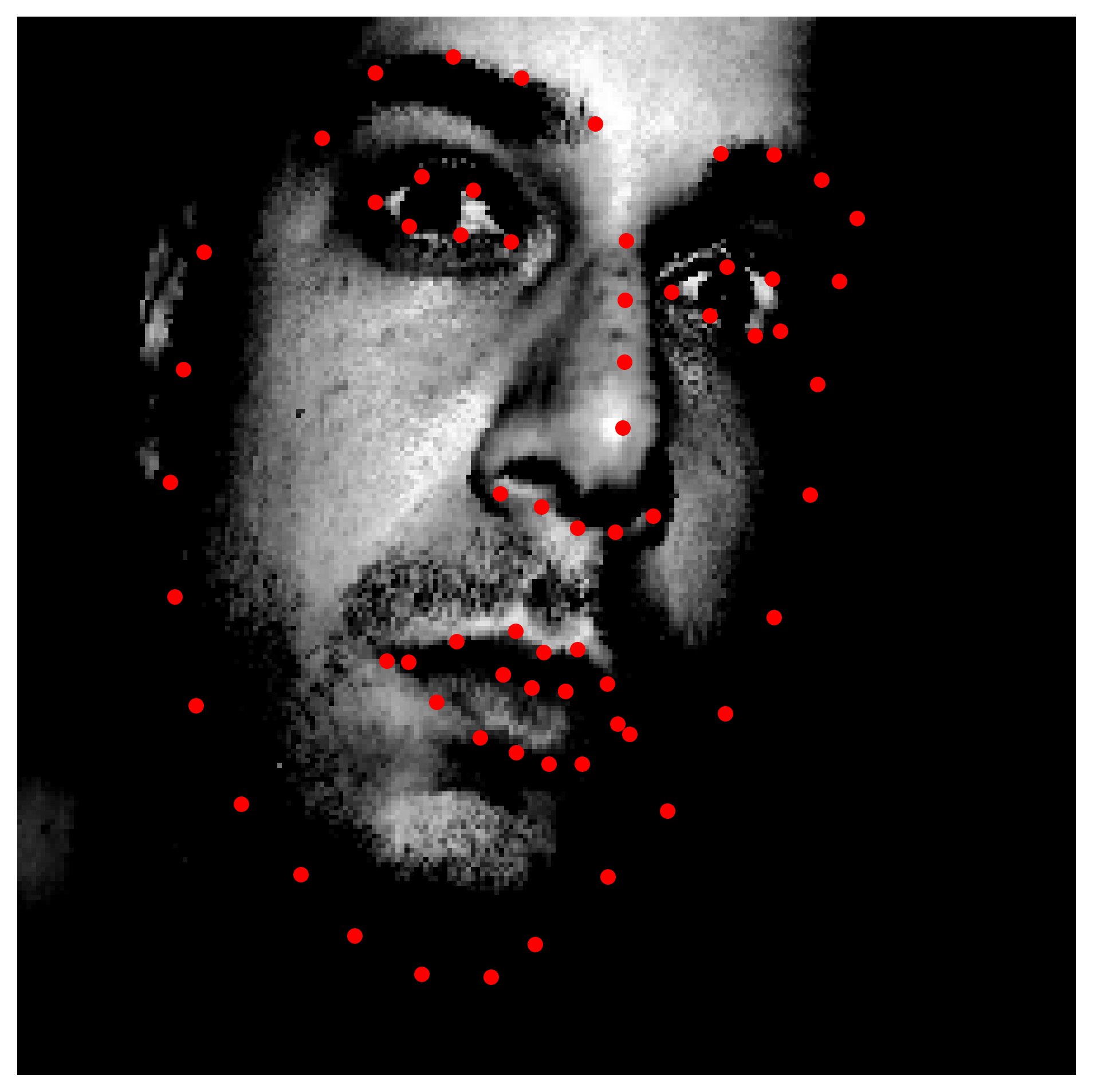
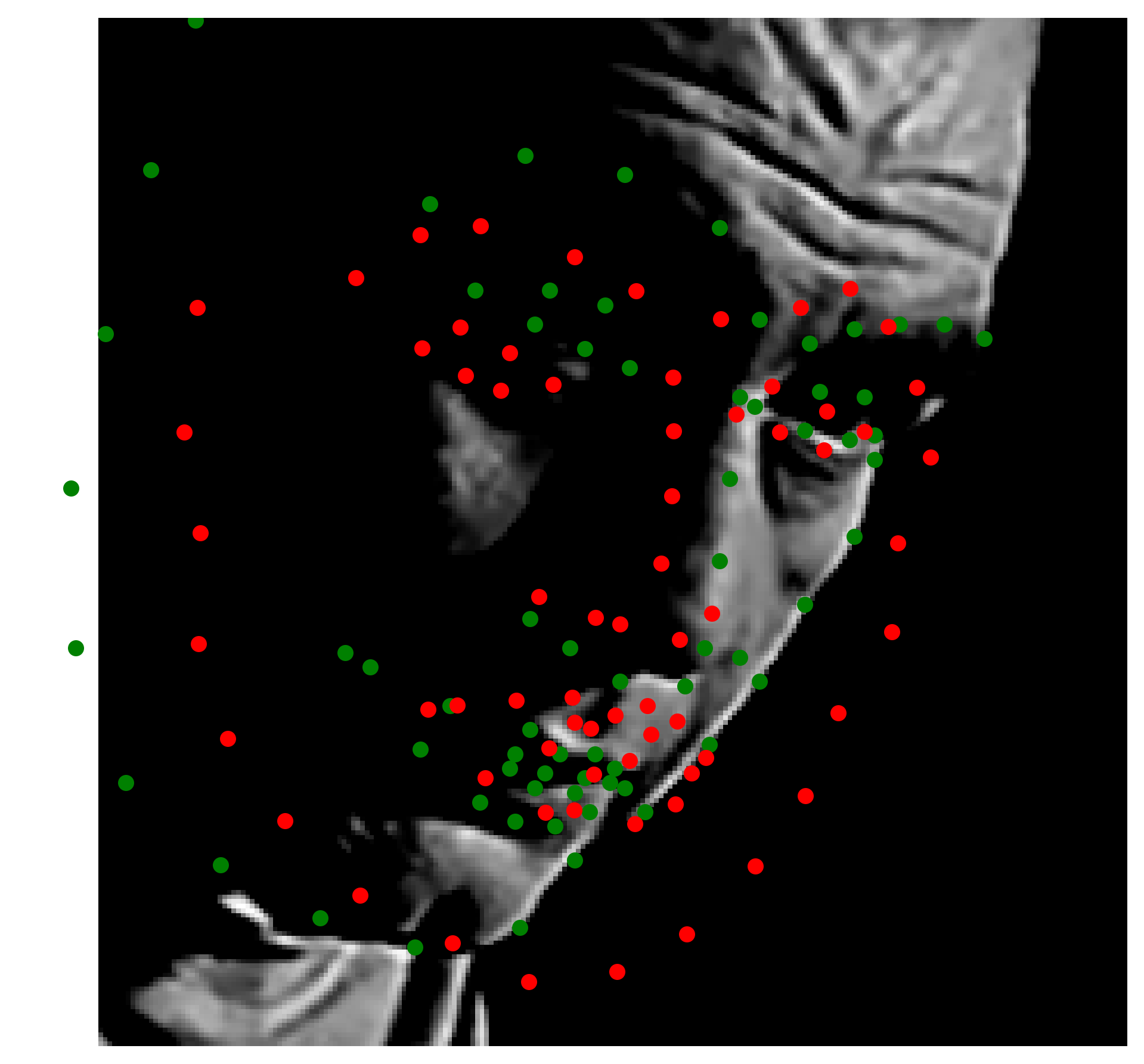
Pixel-wise Landmark Classification
In this part, we are going to turn the problem into a pixelwise classifciation problem from a pixel regression problem. That is, we are going to predict how likely it is for each pixel to be the keypoint. We are going to do so by placing 2D Gaussians over our landmark coordinates.
For this part, we are going to use an U-Net model. The model will take the generated heatmaps as input and generate heatmap predictions. We then have to convert the heatmap predictions to the coordinates of the keypoints. For this, we have initially tested a softmax approach, an argmax approach, and a weighted argmax approach.
The weighted argmax approach works by treating the heatmap predictions as probability distributions over the pixel grid, where the pixel intensities represent the likelihood of a landmark's location. Instead of simply selecting the pixel with the highest intensity (as done in the standard argmax approach), the weighted argmax computes a weighted average of all pixel coordinates, with the heatmap values acting as weights. As the weighted argmax considers the entire heatmap distribution, not just the single most confident pixel, it appeared to provide better results.
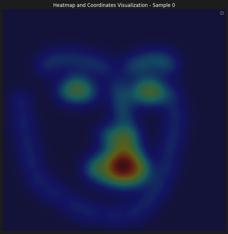
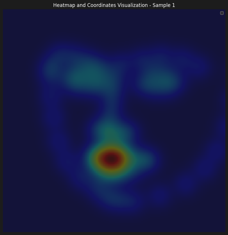
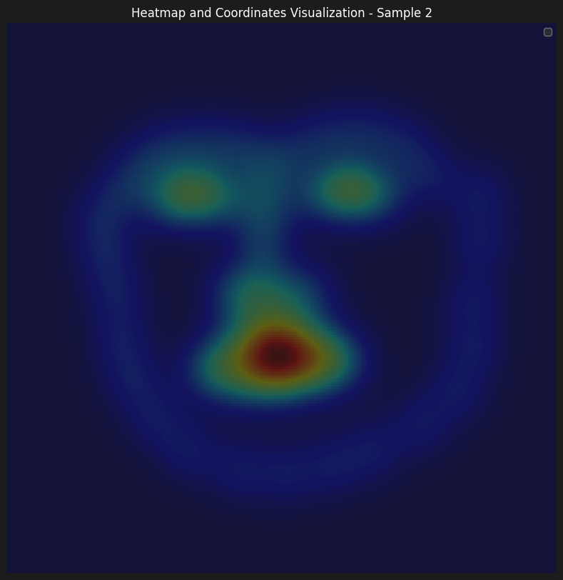
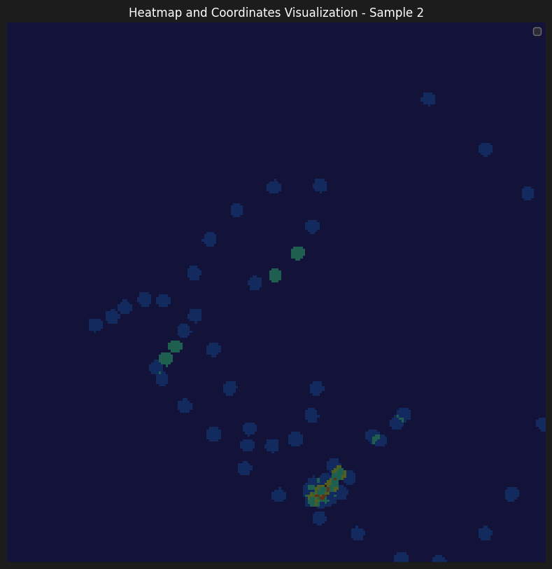
For the generation of the gaussians, we have tried training on sigmas [7, 9, 11]. The larger sigmas turned to overlap the features' heatmaps. We believe this contributed to learning localizing quickly initially, however, the precision of the predictions was not as good as the other sigmas, and the loss converged quickly afterwards. With sigma=7, though loss started higher, we have seen a more consistent learning process.
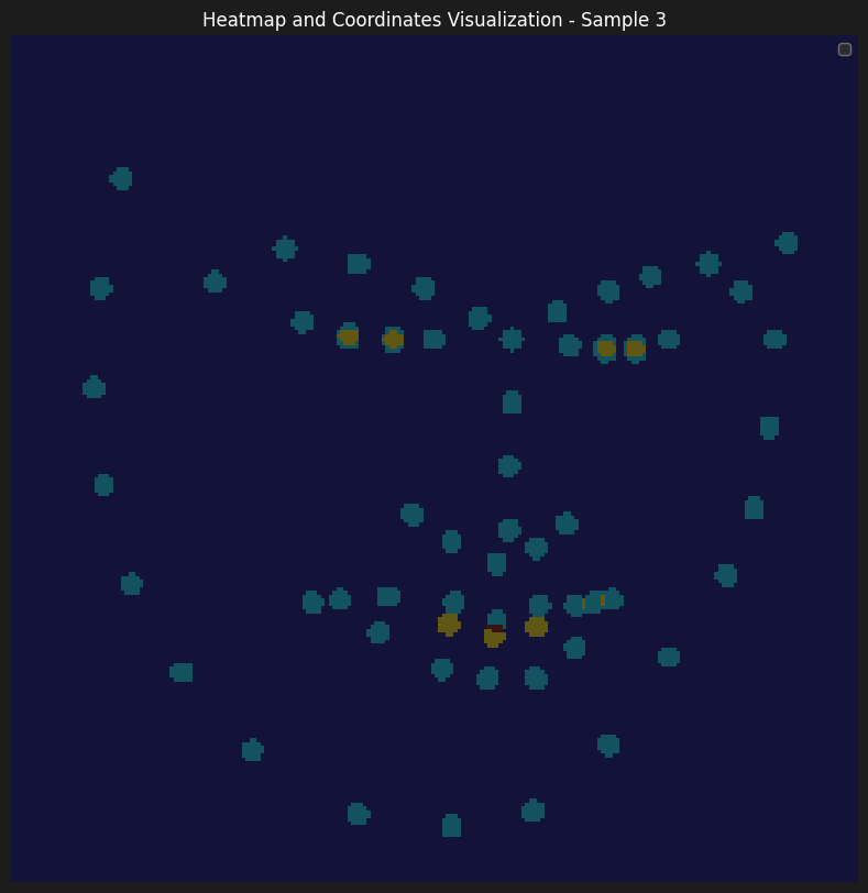
Here are some of the accumulated heatmaps that was used as the input of the model
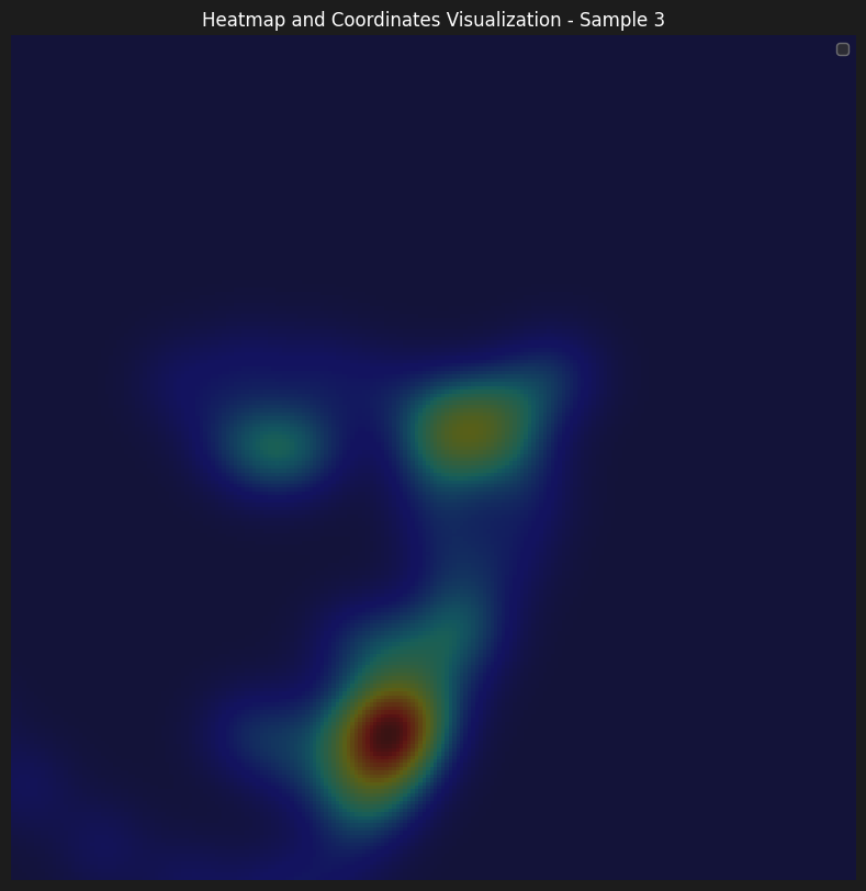
As for the information on the parameters of our training. We have initially started learning with lr=1e-3, although it seemed to learn, the progress was slow. Therefore, we wanted to be able to start from a higher learning rate, however, enable model to make small improvements as the training progressed. That's why, we have implemented a learning rate scheduler with gamma = 0.1 and step size = 5, which enabled us to start with a learning rate of 5e-3.
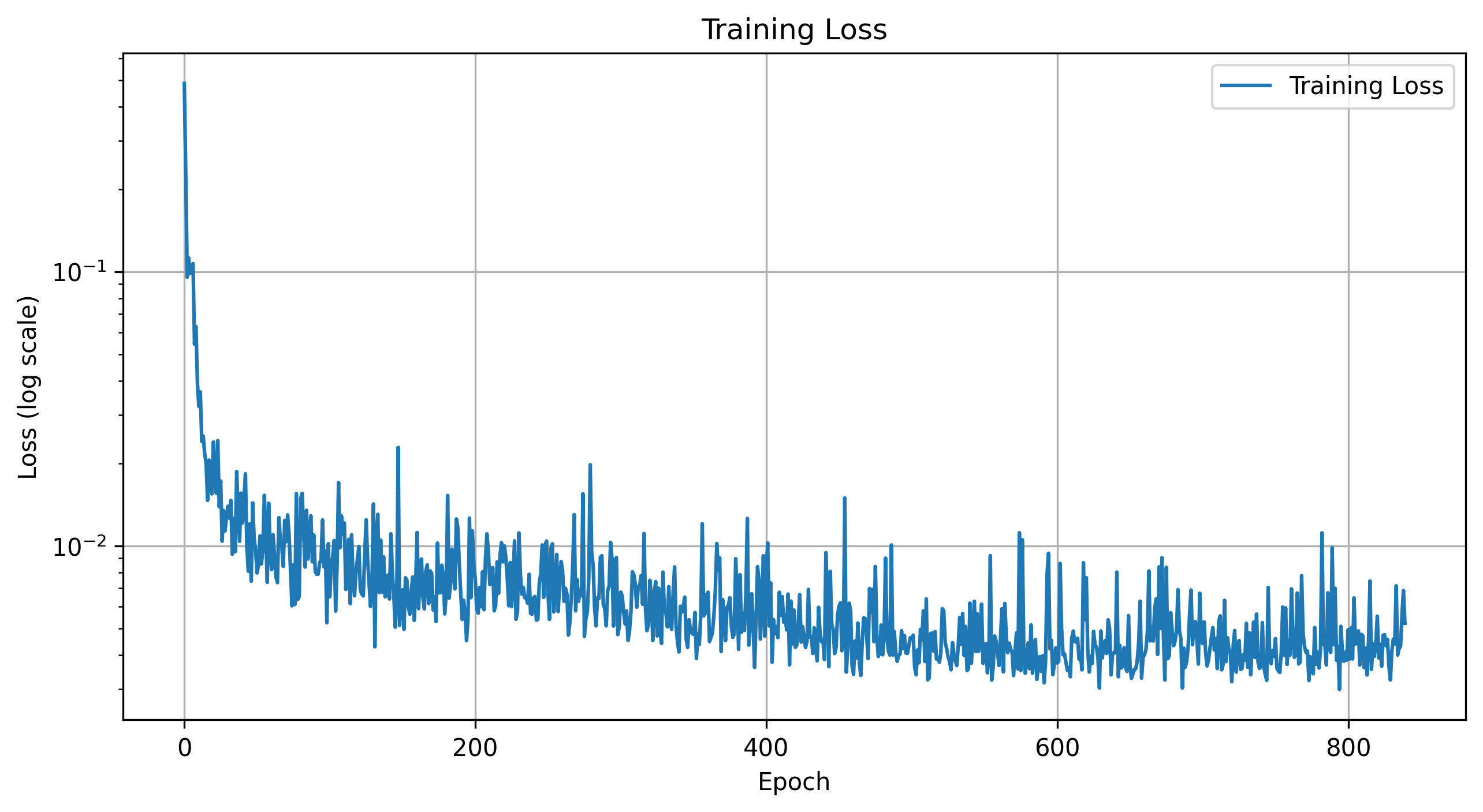
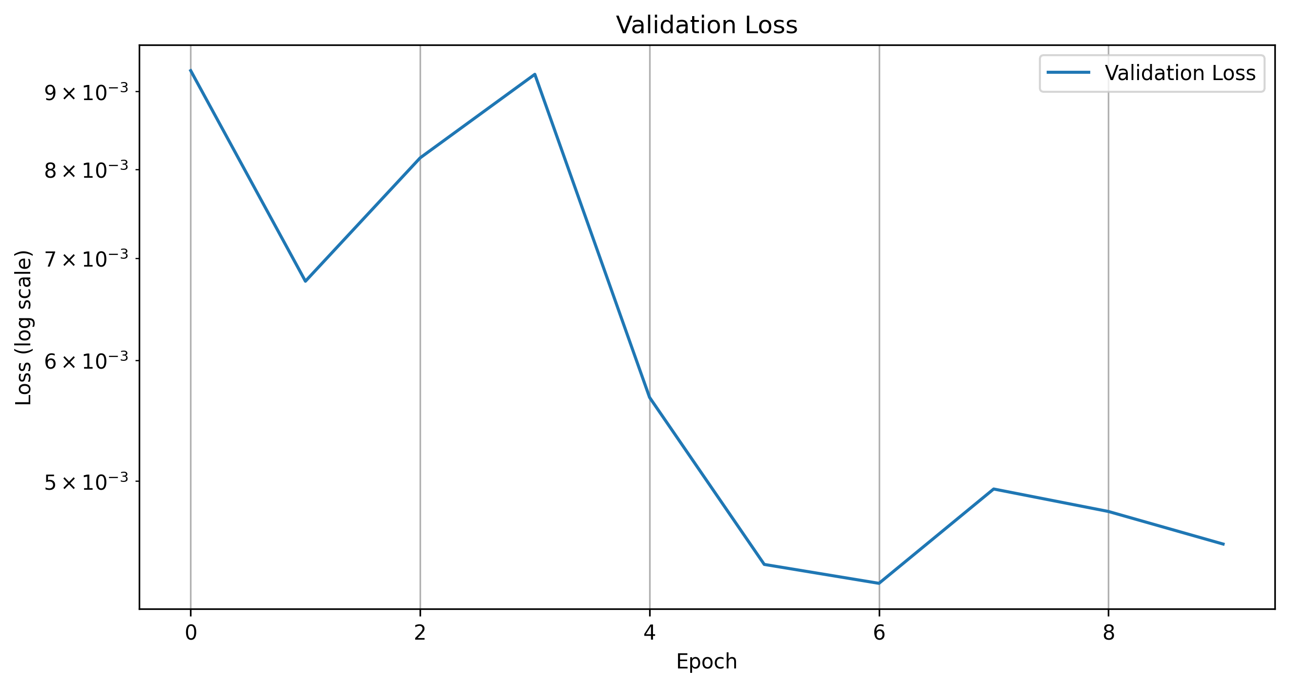
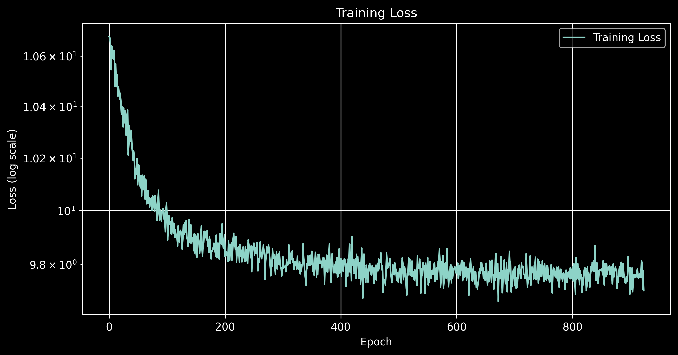
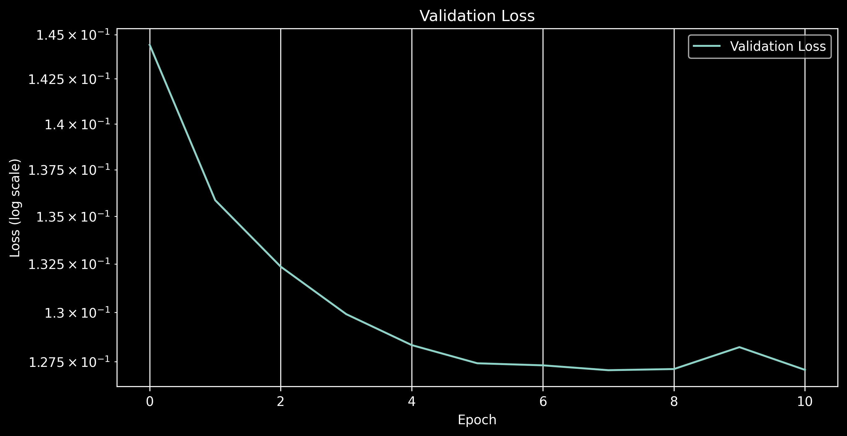
Here are the details of the loss

Training Loss
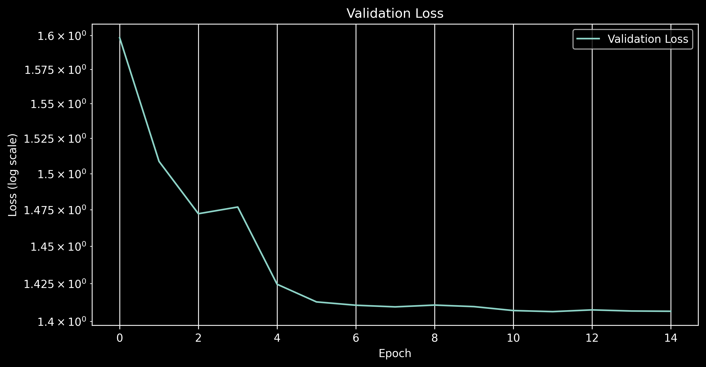
Validation Loss
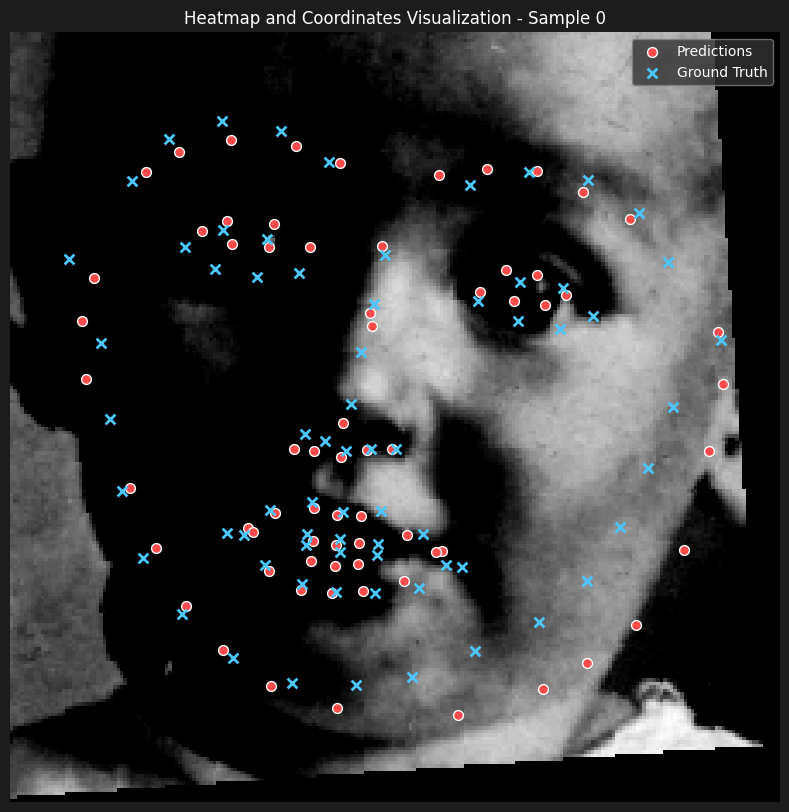
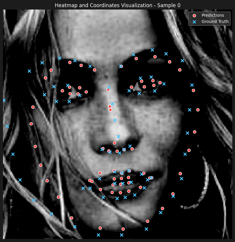
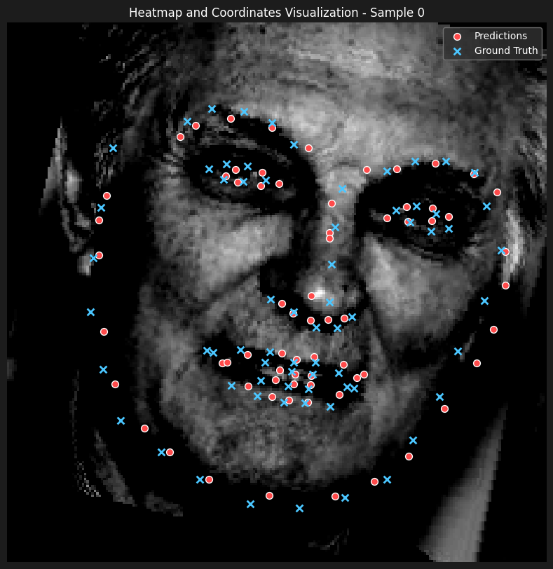
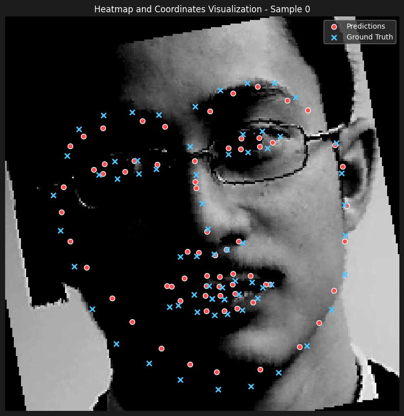
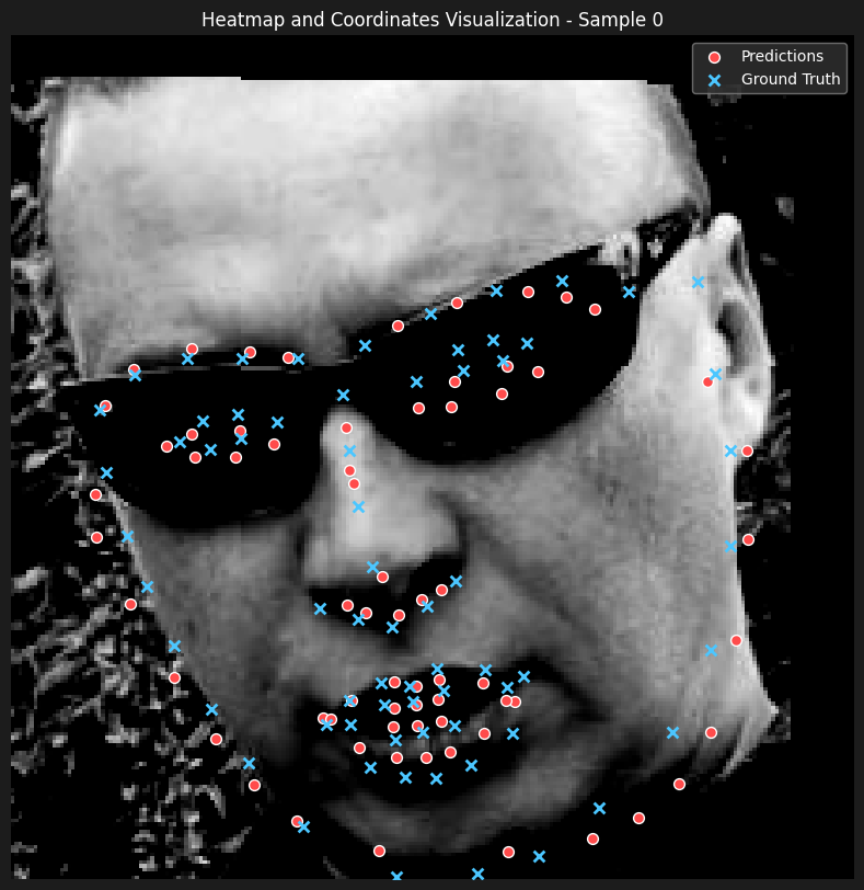
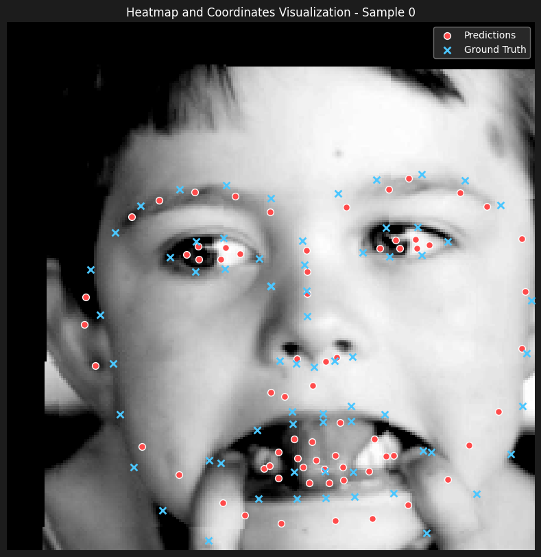
Here are some of the predictions
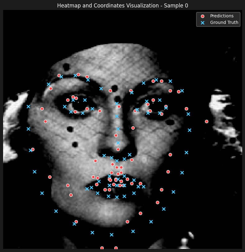
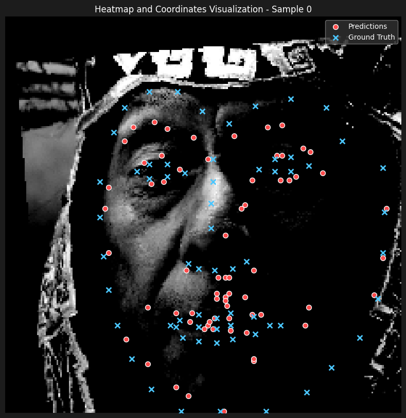
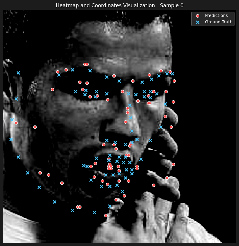
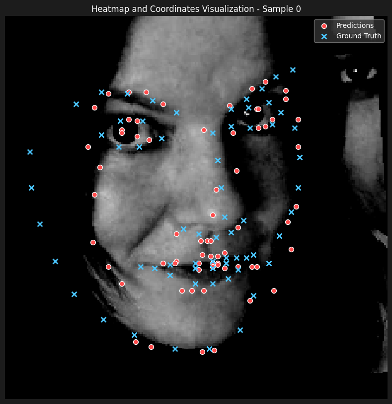
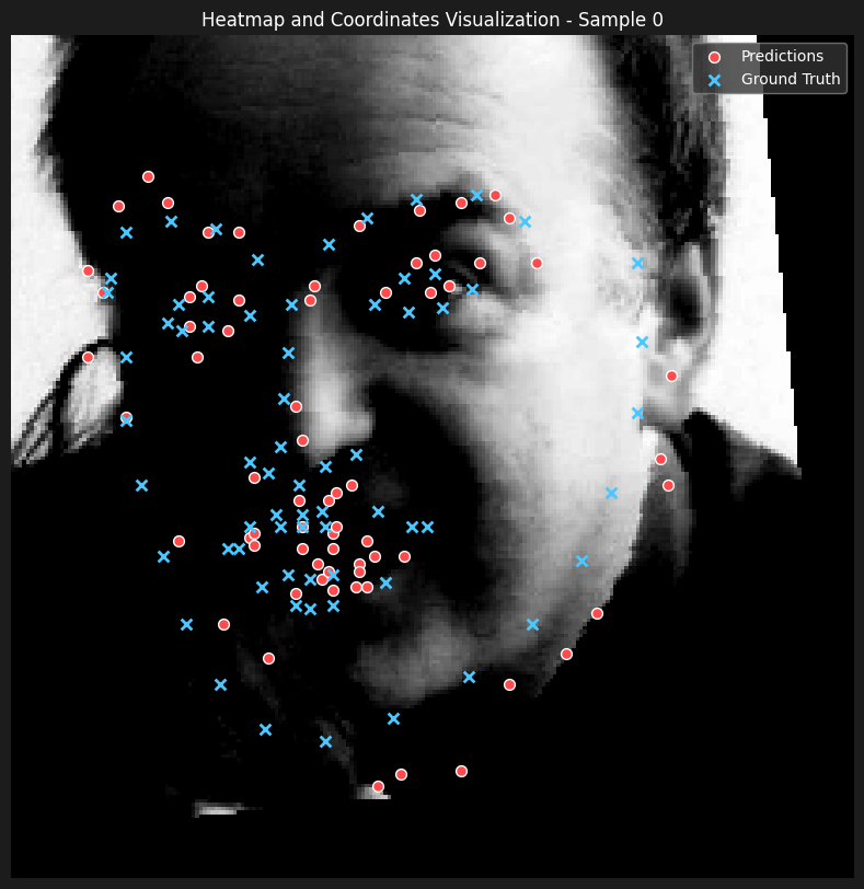
From observing the results, we can see that the model is able to learn the surroinding landmarks of the face pretty accurately, especially compared to inner features such as mouth and nose. Our hyphotesis is that the although it showed satisfactory results to decrease sigma to 7 from 9 and 11, observing the heatmaps, the gaussians seem to overlap quite a lot, which makes it harder for the model to learn the exact location of the landmarks.
BW - Pixel-wise Landmark Classification with 0/1 mask heatmaps.
We wanted to evaluate the results with a 0-1 mask of the heatmaps generated from the coordinates of the landmarks. Since we had the previous deductions regarding the size of the gaussians from last part, we wanted to test this part with masks that have smaller radii, therefore, we used radius=3 for the masks we generated in this part.
Here are some of the heatmaps


As for the training and the model, we have kept everything the same as we deducted that our setup was satisfactory from the previous part. The weighted argmax approach of converting the heatmaps into the coordinates is now equivalent to calculating the centroid of the heatmaps and getting their center of mass to be the coordinates.
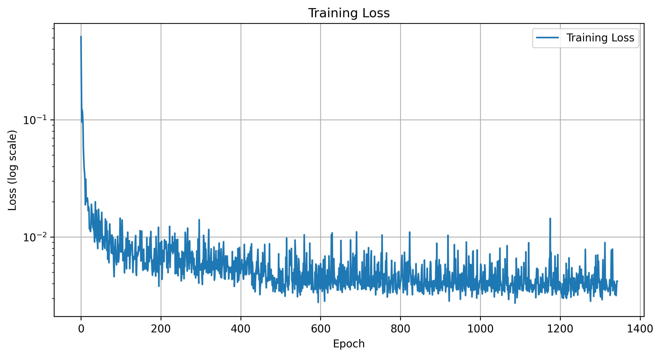
Here is the loss progression
Training Loss
Validation Loss
From the loss progression, we can see a further decrease in the loss compared to the previous Gaussian based approach. Let's observe some of the predictions as well.
Here are some of the predictions
The results seems to be incredibly satisfactory, only output that wasn't as good as the rest of the predictions was a case where the shape of the face was heavily distorted because of the hands pulling the mouth (bottom right).
Though the results are impressive and better than the Gaussian-based approach in this instance, we believe this comparison is not entirely credible. This is because decreasing the radius of the binary mask (compared to the sigma value used for the Gaussian) made a significant difference in our inputs, making the inner face landmarks much more identifiable. Therefore, as we lack a controlled and fair test case, we cannot definitively conclude which approach works better.
However, our intuition aligns with the idea that the Gaussian-based approach would ultimately perform better, particularly with appropriately small sigma values. This intuition stems from the fact that the Gaussian-based heatmaps carry more information about the spatial distribution of a landmark's probability.
Distinction Between Methods:
-
Binary Mask Approach:
When applying the weighted argmax method to a binary mask, the weights are either 1 (inside the mask) or 0 (outside). Mathematically, this reduces to calculating the centroid (center of mass) of the region. Since the weights are uniform, the resulting coordinate is simply the arithmetic average of all pixel locations within the binary mask. No additional spatial information beyond the mask's shape and size is used.
-
Gaussian-Based Approach:
In contrast, the Gaussian-based heatmap encodes a spatial probability distribution around the true landmark location. The pixel values decay smoothly from the center of the Gaussian, assigning higher weights to pixels closer to the landmark and progressively lower weights to pixels farther away.
Mathematically, the weighted argmax for a Gaussian heatmap computes a soft center of mass where the pixel intensities act as probabilities or weights:
                                    xGaussian = (Σ xij * Hij) / Σ Hij,
                                    yGaussian = (Σ yij * Hij) / Σ Hij
Here,
Hijrepresents the Gaussian values at each pixel, which are non-uniform and encode how "likely" each pixel is to be the landmark. This smooth weighting allows the Gaussian-based approach to provide sub-pixel accuracy and more robust predictions, especially when landmarks are partially occluded, ambiguous, or noisy.
Why We Think Gaussian Would Perform Better (in Theory):
In the Gaussian-based method:
- The pixel weights are continuous and smoothly decaying, providing a stronger signal about the landmark's location.
- The weighted average incorporates this probability distribution, which helps the model learn finer spatial relationships and improves landmark localization precision.
In comparison, the binary mask provides only a hard region with equal weight, leading to less spatial information. Therefore, while the weighted argmax reduces to the centroid for binary masks, the Gaussian-based approach leverages richer information to generate more accurate landmark predictions.